Using OpenCV, SciPy, and Scikit-learn to develop a simple Gaelic football tracking system
Published 2020-06-22
Table of Contents
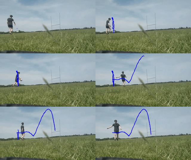
In this blog post I will describe how to implement a simple ball tracking system in Python. We will use the YOLO model and OpenCV to identify and track the ball within each frame. In cases where the model cannot locate the ball, we will use a linear regression model (scikit-learn) and quadratic curve fit (SciPy) to predict the balls location based on it’s trajectory.
While researching OpenCV for this blog post I found Adrian Rosebrock’s blog series extremely useful and would recommend it anyone who is looking to get to grips with the OpenCV library.
Although this blog post focuses on the “key” components of the ball tracking system, I have (as always) made the full code available from my GitHub repository if you wish to step through in detail or run locally.
The YOLO model
The You Only Look Once (YOLO) pre-trained model allows us to perform state-of-the-art object detection in real time. The model supports a wide variety of objects such as bottles, people, elephants, and of course, footballs. While we can run the model on a video (or image) from the terminal, OpenCV allows us to easily implement the YOLO model within python scripts. If you are interested in learning more about the YOLO model, it’s architecture, and it’s performance compared to other models, you can do so here.
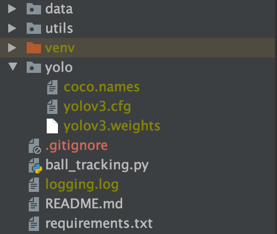
Before we can get stuck into the python side of things we need to download the YOLO architecture (config), weights, and labels. To do this, we first create a yolo/ directory within the project structure (see below). From here, we can download the config from here, the labels here, and the model weights here.
Implement YOLO in OpenCV
Once we have the model files stored locally, we can break the OpenCV/YOLO component of the project up into 3 simple steps:
-
Initialising the YOLO Model
-
Reading the video frames using OpenCV
-
Identifying the balls position within each frame
Initialising the YOLO model
As seen in the function below we will begin by loading the model files and labels. From here we use the OpenCV DNN (deep neural network) method to generate the pre-trained model from the config and weight files.
Next we simply create a list of output layers which we will use to obtain the model outputs later before returning this list along with the model and output labels (which we will also use later).
import cv2
import os

def initialise_yolo():
    """
    Function to initialise the weights, architecture, and labels for the yolo model

    :return: yolo model, yolo model output layer names, model labels (ball, person, etc.)
    """
    yolo_dir = os.path.abspath("./yolo")

    # load the labels, weights, and config for the yolo model
    labels_path = os.path.sep.join([yolo_dir, "coco.names"])
    weights_path = os.path.sep.join([yolo_dir, "yolov3.weights"])
    config_path = os.path.sep.join([yolo_dir, "yolov3.cfg"])

    # load the labels (as list), and model
    labels = open(labels_path).read().strip().split("\n")
    yolo_model = cv2.dnn.readNetFromDarknet(config_path, weights_path)

    # get the output layers
    layer_names = yolo_model.getLayerNames()
    layer_names = [layer_names[i[0] - 1] for i in yolo_model.getUnconnectedOutLayers()]

    return yolo_model, layer_names, labels
Reading the video frames using OpenCV
Perhaps the simplest part of this process, thanks to OpenCV is the processing of individual frames within the input video. To do this we simply create a video stream object (as seen below) using our input video. From here we can implement a simple while loop to iterate through each frame while there is a frame to load from the original video.
To speed things up, we can also use the imutils library to downsize each frame in our input video. Of course, depending on the processing power of you machine, you may choose to ignore this step.
import cv2
import imutils

vs = cv2.VideoCapture(INPUT_VIDEO_PATH)

while True:
    # grab the next frame in the video stream
    (grabbed, frame) = vs.read()

    # check to see if we have reached the end of the stream
    if frame is None:
        break

    # resize the frame (so we can process it faster)
    frame = imutils.resize(frame, width=500)
    (H, W) = frame.shape[:2]
Identifying the balls bounding box within each frame
Once we have the YOLO model initialised, and a mechanism for iterating over video frames in place, we are ready to start tracking the ball.
As demonstrated below, we begin by converting each frame to a blob (a 4-d matrix) using OpenCV’s blobFromImage method. We then pass the blob through the YOLO model and collect the values from the model’s output layers. Next we iterate through these outputs and for each object detected in the frame that is above our defined confidence threshold (0.3 in my case), we determine that objects bounding box information.
From here, we apply a non-maxima suppression to get a more accurate bounding box for each object detected in the frame before finally filtering and identifying the bounding box for the “sports ball” object*. Of course if there are more objects you want to track, you can filter down to those too.
# use the yolo model to detect objects in image and get their bounding boxes
blob = cv2.dnn.blobFromImage(frame, 1 / 255.0, (416, 416), swapRB=True, crop=False)
yolo_model.setInput(blob)
layerOutputs = yolo_model.forward(ln)
boxes = []
confidences = []
classIDs = []

for output in layerOutputs:
    # loop over each of the detections
    for detection in output:
        # get the class id and confidence for the object
        scores = detection[5:]
        classID = np.argmax(scores)
        confidence = scores[classID]

        if confidence > confidence_threshold:

            # get the bounding box for the object
            box = detection[0:4] * np.array([W, H, W, H])
            (centerX, centerY, width, height) = box.astype("int")
            # use the center (x, y)-coordinates to derive the top and and left corner of the bounding box
            x = int(centerX - (width / 2))
            y = int(centerY - (height / 2))
            # update our list of bounding box coordinates, confidences, and class IDs
            boxes.append([x, y, int(width), int(height)])
            confidences.append(float(confidence))
            classIDs.append(classID)

# apply non-maxima suppression to refine the balls bounding box
idxs = cv2.dnn.NMSBoxes(boxes, confidences, confidence_threshold, suppression_threshold)

# ensure at least one detection exists
if len(idxs) > 0:
    # loop over the indexes we are keeping
    for i in idxs.flatten():
        # we only care about the ball
        if labels[classIDs[i]] == "sports ball":

            # let the system know we found the ball
            ball_found_initially = True
            ball_found_in_frame = True
            object_lost_count = 0
            prediction_count = 0

            # extract the bounding box coordinates
            (x, y) = (boxes[i][0], boxes[i][1])
            (w, h) = (boxes[i][2], boxes[i][3])
            # calculate the centre of the bounding box to draw the trace on the frame
            trace_location = (int(x + (w / 2)), int(y + (h / 2)))
Note: It’s probably a bit inefficient how I do this in the code. I should probably only calculate the bounding box and perform non-maxima suppression on the objects I want (i.e. the football). Since my example video files don’t contain many other labels the YOLO model can identify, it shouldn’t slow things down too much. However if you were doing this in a “real” setting I would recommend trying to be more efficient here.
Predicting ball trajectory using SciPy and Scikit-learn
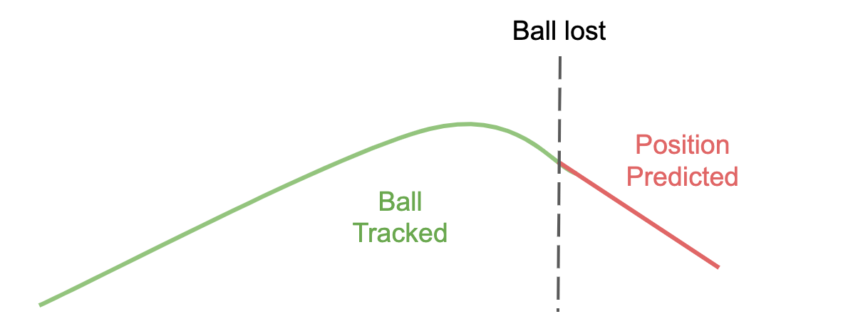
Of course, due to the quality of our recording equipment, the distance the ball is from the camera, or lighting, the model may lose track of the ball from time to time. To overcome this, we can use a very simple two step approach to predict the position of the ball within the frame, based on it’s trajectory in the previous 20 frames (of course you can change this number):
-
Use a linear regression model to predict the balls x position
-
Determine the y position based on the curve fitted to the proceeding x-y coordinates
Predicting the x position using linear regression
Nothing too crazy here, we simply take the last 20 x coordinates, their times i (in range 0-19) and fit a linear regression model. Once fit we predict the x position by passing in i = 20 to the model.
from sklearn.linear_model import LinearRegression

x_train = [pt[0] for pt in tracked_points]
x_train.reverse()

# fit a simple linear regression model to predict the next x position
x_train = x_train[-20:]
times = [i for i in range(len(x_train))]

reg = LinearRegression().fit(
    np.array(times).reshape(-1, 1), np.array(x_train).reshape(-1, 1)
)
x = reg.predict(np.array([20]).reshape(1, -1))[0]
Determine y position using a curve fit
Once we have our predicted x positions, we can make a prediction for the y coordinate of the ball by solving the quadratic equation given by the balls position in the previous 20 frames. I chose to use a quadratic equation as it is a function which represents a typical ball trajectory.
Before we use SciPy to calculate the functions constants, we must define our quadratic function in the form of a python function.
def quadratic_eqn(x, a, b, c):
    return (a * (x * x)) + (b * x) + c
Once defined, we can fit this quadratic function using SciPy’s curve_fit function to obtain values for a, b, and c in the equation above. We can then pass these values, and our predicted x position to our quadratic equation python function to solve for y and obtain our predicted ball location.
y_train = [pt[1] for pt in tracked_points]
y_train.reverse()

# obtain values for a, b, c
popt, pcov = curve_fit(quadratic_eqn, np.array(x_train[-20:]), np.array(y_train[-20:]))

# use our curve fit to predict the next y
y = quadratic_eqn(x, popt[0], popt[1], popt[2])

trace_location = (int(x + (w / 2)), int(y + (h / 2)))
Writing frames to output file
Once we have detected the ball in the frame, or have made a prediction based on its trajectory, all that is left is for us to trace the balls position onto the frame and write it to an output file.
We can draw the trajectory line by iterating over our list of tracked points (for each frame) and drawing a line connecting them using openCv’s line method. The example below will draw a blue line of width 2 connecting each point. It is worth noting that this action will update the frame we are iterating over.
# loop over the set of tracked points
for i in range(1, len(tracked_points)):
    # if either of the tracked points are None, ignore them
    if tracked_points[i - 1] is None or tracked_points[i] is None:
        continue
    # otherwise, draw a line connecting them
    cv2.line(frame, tracked_points[i - 1], tracked_points[i], (255, 0, 0), 2)
From here we can initialise the video writer object (if not done already) and write our updated frame to the output file (e.g. example.mp4)
# write the frame to our output file
if writer is None:
    # initialize our video writer
    writer = cv2.VideoWriter(
        output_location,
        cv2.VideoWriter_fourcc('m', 'p', '4', 'v'),
        30,
        (frame.shape[1], frame.shape[0]),
         True
    )

# write the output frame to disk
writer.write(frame)
Once we have processed each frame in our input video we can close our video stream and writer objects using the release method.
writer.release()
vs.release()
Bringing it all together
As mentioned in the introduction, this blog post covers the key components required to implement a simple ball tracking system. While I have the full code available from my GitHub repository, I have summarised the process below in pseudocode to give you a better understanding of how it all comes together:
load input video file
for frame in input
	process frame through yolo
	if ball found
		obtain ball location
		ball lost counter = 0
	else;
		ball lost counter +1
	if (ball lost counter = 10) and frame number
		predict ball location
	for point in ball locations
		draw line
	write to output
close stream and writer objects
Future directions
Although this blog post describes how we can implement a simple ball tracking system using OpenCV, there are a number of ways the system could be improved and expanded upon:
-
Improving the camera used to record the video (I was using the camera on my phone) could be an easy way to improve the YOLO models ability to track the ball throughout the entire video
-
Use an additional camera positioned behind or under the goal post to automatically identify if a goal or a point is scored
-
Use the “person” label available within YOLO to only begin tracking the ball once it leaves the player’s foot
-
Improve the trajectory prediction component by using a more sophisticated modelling approach (maybe deep learning) and more data (trajectories from other shots tracked using the system)