Using general linear models to simulate Gaelic football matches in python

Published 2020-10-16

In this blog post I will describe how we can use our understanding of the normal and poisson probability distributions to simulate Gaelic football matches for Dublin’s division 1 adult football league and determine the probability of either team winning the match.

I will begin by briefly summarising the rules of the game and how we can download the data required from the Dublin GAA’s website. From here I will discuss the normal and poisson distributions and how they can be used to calculate expected goals and points in a given match. Finally I will bring it all together and demonstrate how we can use these distributions to simulate matches and calculate win probabilities.

As always, if you would prefer a more interactive tutorial I have prepared a jupyter notebook version of this tutorial which is available from my GitHub repo.

A brief summary of Gaelic football and it’s scoring system

In case you are reading this blog and have no knowledge of Gaelic football, I will attempt to briefly summarise the sport and it’s scoring system so you will have all the information required to continue with this tutorial.

Gaelic football is a sport where two teams of 15 play against each other to try accumulate the most points over the course of the match. Players can carry the ball with their hands but must bounce, or solo (drop the ball onto their foot and back up to their hand) every 4 steps.

When it comes to scoring, teams can score in 2 ways:

1. Kicking the ball into the net for a goal – this is worth 3 points
2. Kicking or punching the ball over the crossbar for a point – this is worth one point

If you wish to learn more about the rules of Gaelic football, you can do so here.

Import data

The data used as part of this analysis was scraped from the latest results section of the Dublin GAA website and has results from all matches the played in Dublin’s senior adult division 1 league during the 2019 season. Rather than going into detail on this, as there is a lot to get through, I will summarise by saying that I essentially iterated through each row of the table (displayed in figure 1) on this website and pulled the scores for each match before saving them to the dataframe that I read in using pandas below.

This dataframe contains the results of all 99 fixtures from the 2019 division 1 season. It’s worth noting that this is a pretty small results dataset but it will be enough for us to use when building some simulation models.

Once the data is read in, I create total_goals and total_points columns for each match. These columns will be used in the next section to understand how goals and points are distributed across games and will inform our modelling decisions later on.

If you would like more detail on how the data was scraped, I have prepared a jupyter notebook which goes through the steps involved in scraping the data and it is available within the git repo supporting this tutorial.

Understanding how goals and points are distributed

Before we can get stuck into any modelling, we will have to take a look at how points and goals are distributed across matches. For example while expect that points will be distributed normally, it is important that we confirm this as if they are actually distributed according to a poisson distribution and we fit a model under the assumption that they are normally distributed, our simulation results will be inaccurate.

To do this we can use a goodness of fit test between the expected distribution, and the actual to determine if they differ significantly.

Point distribution

Taking a look at the distribution of points across games visualised below (figure 2), we can see that the distribution is very similar to the normal distribution overlaid in red. Of course it does not match exactly, however given the reasonably small sample size of games, that is understandable.

When we take a look at the goodness of fit test between the points distribution and the normal distribution, performed by using scipy’s ks_2samp function we can see that the p-value is much greater than 0.05 and as a result of this we can assume going forward that our points data is normally distributed.

mean_points = gaa_df['total_points'].mean()
points_std = gaa_df['total_points'].std()
normal_dist = np.random.normal(mean_points, points_std, 100000)
 
ks_2samp(np.array(gaa_df['total_points']), normal_dist)
 
# Output
>>> Ks_2sampResult(statistic=0.0937287878787878, pvalue=0.34992454962173847)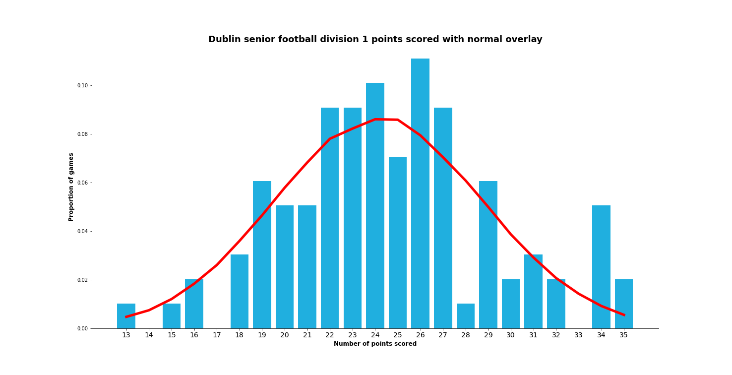

Goal distribution

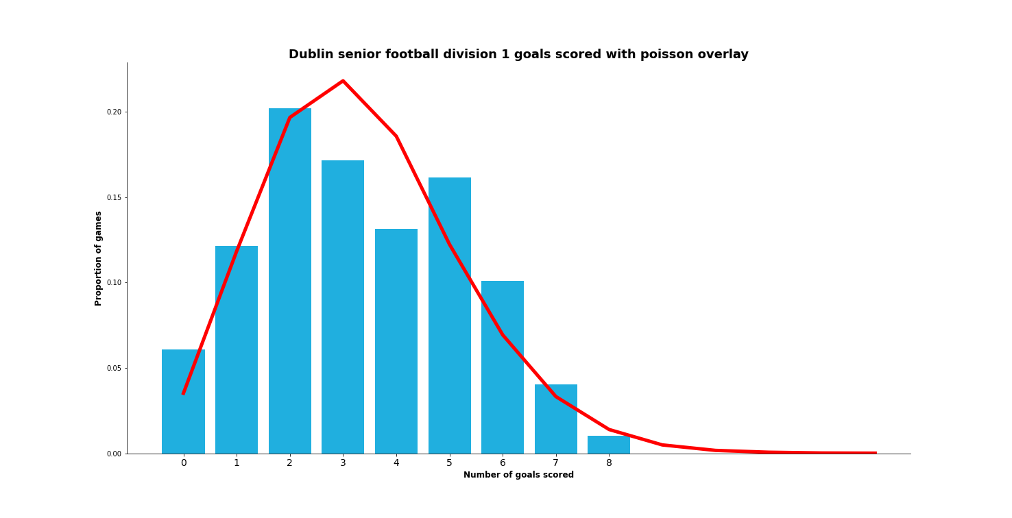
Conversely, when we take a look at our goal distribution (figure 3) we can see that they appear to be distributed according to a poisson distribution, and in fact when we take a look at the goodness of fit test for this we can once again see a high p-value which indicates that goals are in fact distributed according to a poisson distribution.

This comes as no surprise as occurrence of goals in similar, more widely researched sports such as soccer are also distributed according to a poisson distribution.

mean_goals = gaa_df['total_goals'].mean()
poisson_dist = poisson.rvs(mean_goals, size=100000)
 
ks_2samp(np.array(gaa_df['total_goals']), poisson_dist)
 
 
# Output
>>> Ks_2sampResult(statistic=0.06953131313131311, pvalue=0.725358743958155)
 

Making some simple predictions for goals & points scored

Now that we understand how goals and points are distributed, we can use this information to make some simple predictions of how many goals or points a team is expected to score in a given match using the cumulative density (for normal distribution) and probability mass (for poisson) functions.

Some preliminary data preparation

Before we get stuck into this, we will perform a bit of data transformation to get our GAA dataset into a format that will allow us to calculate each teams average goals and points a bit easier.

To do this we will simply split the data into home and away dataframes and create a row for each teams performance per game as well as who their opponent was and their performance before creating an at_home flag which we will use a bit later for our more advanced model.

home_df = gaa_df[[
    'game_id', 'date', 'time', 'location', 'home_team', 'home_team_goals', 'home_team_points', 'away_team', 'away_team_goals', 'away_team_points'
]]
 
away_df = gaa_df[[
    'game_id', 'date', 'time', 'location', 'away_team', 'away_team_goals', 'away_team_points', 'home_team', 'home_team_goals', 'home_team_points'
]]
 
home_df['at_home'] = 1
away_df['at_home'] = 0
 
home_df.columns = away_df.columns = [
    'game_id', 'date', 'time', 'location', 'team', 'team_goals', 'team_points', 'opponent', 'opponent_goals', 'opponent_points', 'at_home'
]
 
team_results_df = pd.concat([home_df, away_df])
team_results_df.head()
 

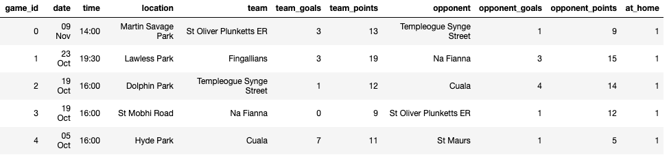
Once we have the data in this format we then calculate each teams average goals and points scored using a pandas aggregation.

team_averages = team_results_df.groupby('team')[['team_goals', 'team_points']].mean().reset_index()
team_averages.columns = ['team', 'average_goals', 'average_points']
team_stds = team_results_df.groupby('team')[['team_goals', 'team_points']].std().reset_index()
team_stds.columns = ['team', 'goals_std', 'points_std']
team_averages = team_averages.merge(team_stds, on = 'team')
team_averages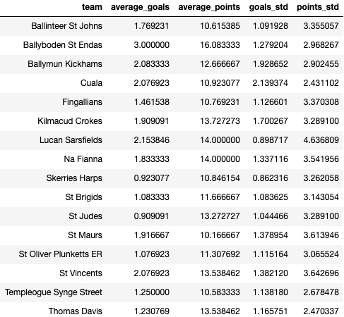

Predicting point probabilities using the normal distribution and it’s cumulative density function

Since we are comfortable that our points data is normally distributed we can calculate a basic probability that a team will score less than x points given the average number of points they usually score, and their standard deviation.

From a theoretical perspective, we do this by first calculating the Z score of observing up to x points given the mean (μ) and standard deviation (σ) where:

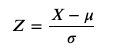
From here we look up this Z value in a set of stats tables to determine the probability of observing up to this value (Φ(𝑍)) such that:

Example:

What is the probability that Ballyboden St Endas will score less than 16 points in a game?

Here we know that 𝑋=16 , 𝜇=16.083 , 𝜎=2.968 .

So:

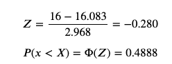
In other words there is a probability of 0.49 that Ballyboden will score less than 16 points in a game.

Why only less than?

By default the Z score/p-value approach returns the cumulative probability of observing a result (points scored) less that 𝑋 . However if instead we want to calculate the probability that Ballyboden scores 16 or more points we can very easily do this by subtracting the probability of scoring less than 16 from 1 as seen below:

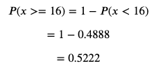
What if I want to calculate exact point probabilities?

Unfortunately since the normal distribution is a continuous distribution, the probability of observing a particular exact value is 0. We can however calculate the probability of observing a value within a given range.

For example, if we wanted to calculate the probability of Ballyboden scoring 16 points we could consider this the same as the probability of them scoring between 15.5 and 16.5 points. When we think of it like this, the calculation becomes a lot easier:

Examples using python

Thankfully for us, scipy’s norm function allows us to quickly calculate the probability of observing particular values in a normal distribution.

In the below examples you will see how we can use this function, along with our data to answer some point probability questions.

Whats the probability of Ballyboden scoring less than 16 points in a game?

team = 'Ballyboden St Endas'
score_less_than = 16
 
team_avergage = team_averages.loc[team_averages['team']==team, 'average_points'].values[0]
team_std = team_averages.loc[team_averages['team']==team, 'points_std'].values[0]
 
probabiltity = norm(team_avergage, team_std).cdf(score_less_than)
print(f"Probability: {round(probabiltity, 4)}")

What's the probability of Ballymun scoring more than 15 points in a game?

team = 'Ballymun Kickhams'
score_more_than = 15
 
team_avergage = team_averages.loc[team_averages['team']==team, 'average_points'].values[0]
team_std = team_averages.loc[team_averages['team']==team, 'points_std'].values[0]
 
probabiltity = 1 - norm(team_avergage, team_std).cdf(score_more_than)
print(f"Probability: {round(probabiltity, 4)}")

Whats the probability of Na Fianna scoring more than 14.5. and less than 15.5 points in a game?

team = 'Na Fianna'
score_more_than = 14.5
score_less_than = 15.5
 
team_avergage = team_averages.loc[team_averages['team']==team, 'average_points'].values[0]
team_std = team_averages.loc[team_averages['team']==team, 'points_std'].values[0]
 
probabiltity_more_than = norm(team_avergage, team_std).cdf(score_more_than)
probabiltity_less_than = norm(team_avergage, team_std).cdf(score_less_than)
print(f"Probability: {round(probabiltity_less_than, 4) - round(probabiltity_more_than, 4)}")

Predicting goal probabilities using the poisson distribution and it’s probability mass function

Similarly to the normal distribution, the poisson distribution also allows us to calculate the probability of scoring a particular number of goals given the team’s mean number of goals scored. However unlike the normal distribution, the poisson distribution is a discrete distribution which means we can calculate the probability of scoring an exact number of goals.

To calculate the probability of scoring 𝑥 goals according to the poisson distribution, we can use the following formula:

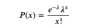
Where 𝜆 the average number of goals scored by the team per game.

Example:

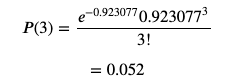
What is the probability that Skerries Harps score 3 goals in a match?

Probability of scoring more than N goals?

If we want to calculate the probability that a team will score 2 or more goals, this would simply be 1 minus the probability of scoring 0 or 1 goals:

Examples using Python

Similar to before, scipy has a handy poisson function which allows us to easily calculate these probabilities as demonstrated in the examples below

What is the probability of Skerries Harps scoring 3 goals in a match?

team = 'Skerries Harps'
number_of_goals = 3
 
team_avergage = team_averages.loc[team_averages['team']==team, 'average_goals'].values[0]
 
probabiltity = poisson.pmf(number_of_goals, team_avergage)
print(f"Probability: {round(probabiltity, 4)}")

Whats the probability of Fingallians scoring more than 2 goals in a match?

team = 'Fingallians'
 
team_avergage = team_averages.loc[team_averages['team']==team, 'average_goals'].values[0]
 
probabiltity = 1 - (poisson.pmf(0, team_avergage) + poisson.pmf(1, team_avergage) + poisson.pmf(2, team_avergage))
print(f"Probability: {round(probabiltity, 4)}")

Calculating expected goals & points taking into account the opponent and home field advantage

While the simple approach described above can help us get to grips with the normal/poisson distributions and the idea of predicting goal probabilities, it fails to take into account the quality of the opponent and any home field advantage which may be in play.

We can get around this however by fitting a normal/gaussian regression model for points (since the response variable is normally distributed), and poisson regression model for goals to predict the expected number of points/goals a team will score against a particular opponent with home field advantage in mind.

Of course we can add any number of variables to this model (e.g. average passes per team, possession, etc.) as they are available, however for the purposes of this tutorial the three mentioned above will suffice.

Thankfully for us, we can very easily fit a normal or poisson regression using the statsmodels library, as demonstrated below.

Points – normal regression

We can fit a regression model to predict the number of points a team will score against a particular opponent by passing in the variables from the team_results_df we created earlier and specifying the family as sm.families.Gaussian().

normal_model = smf.glm(
    formula="team_points ~ at_home + team + opponent", data=team_results_df, family=sm.families.Gaussian()
).fit()
 
normal_model.summary()

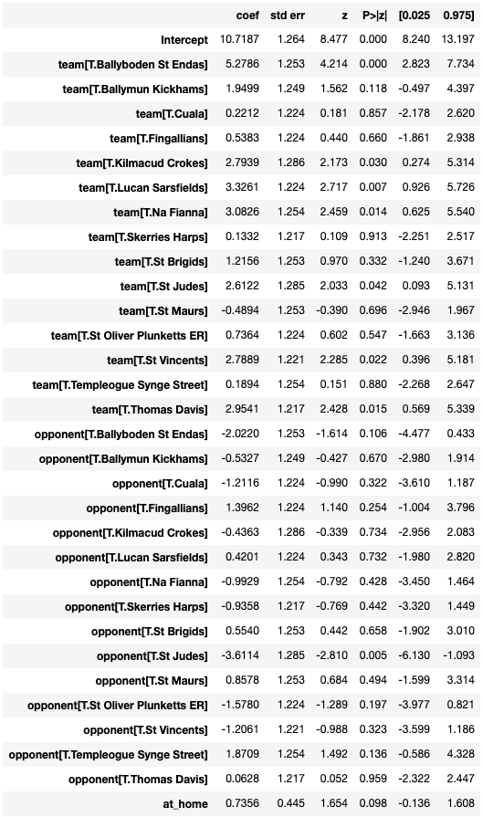
When we take a look at the output below, the first thing that we notice is that there is a lot of information. However for the purposes of understanding how the predictions will work, the main things we are interested in are the values in the coeff column. These values represent what we will pass into the regression model formula to calculate the expected goals a team will score.

Example:

Consider we want to put a bet on how many points Ballymun Kickhams will score in a home fixture against Lucan Sarsfields. We would begin by pulling the intercept(always included), team[T.Ballymun Kickhams], opponent[T.Lucan Sarsfields], and at_home values from the table below (note if the team you want to determine the expected points for is playing away you can leave out the at_home value).

From here, we can simply plug these in to the normal regression formula:

Where 𝜃x is the sum of our coefficient values (including the intercept).

Doing this we get:

Using this data, our model tells us that Ballymun are expected to score 13.82 points against Lucan.

Of course we don’t always have to do this by hand as statsmodels provides a predict() function which we will use in our simulations (see below).

normal_model.predict(
    pd.DataFrame(data={'team': 'Ballymun Kickhams', 'opponent': 'Lucan Sarsfields', 'at_home':1},index=[1])
).values[0]
 
# Output
>>> 13.824284078685377

Goals – poisson regression

As with the points data, we can simply fit a poisson regression model using the same variables to make a prediction on the number of goals a team is expected to score against a particular opponent.

poisson_model = smf.glm(
    formula="team_goals ~ at_home + team + opponent", data=team_results_df, family=sm.families.Poisson()
).fit()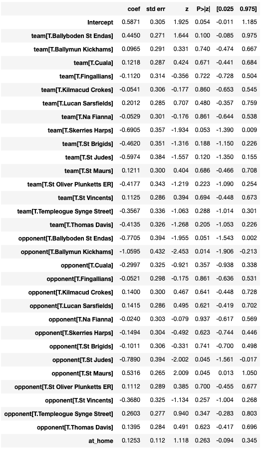

Example:

Instead of points, let’s say we want to know how many goals Ballymun should score against Lucan. Well the process is very similar, and as with before we begin by pulling the intercept, team[T.Ballymun Kickhams], opponent[T.Lucan Sarsfields], and at_home values from the table below.

From here, we plug these values into the slightly different poisson regression formula:

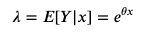
Where once again 𝜃x is the sum of our coefficient values (including the intercept).

Doing this we get:

Calculating the above we can see that our models expects Ballymun to score 2.58 goals against Lucan. This combined with the 13.82 points predicted above should surely be enough to get them the win!

Once again, we can use the predict() function to perform these calculations easily in python.

poisson_model.predict(
    pd.DataFrame(data={'team': 'Ballymun Kickhams', 'opponent': 'Lucan Sarsfields', 'at_home':1},index=[1])
).values[0]
 
# Output
>>> 2.5863274203336766

A note on interpreting the coefficient values

1. You will notice that Ballinteer St Johns don’t appear anywhere in this summary. This is because they appear first alphabetically in the data and are thus considered to be the intercept for the model. You can think of all other coefficient values as that teams attacking of defensive strength compared to Ballinteer. For example if a team has a positive coefficient value, it will mean they are a superior attacking team to Ballinteer, whereas a team with a negative coefficient can be considered inferior as an attacking threat. Conversely, an opponent with a positive coefficient can be considered a worse team defensively, while an opponent with a negative coefficient can be considered a better defensive team.

2. With point 1 in mind, we can use the coefficient values to rank teams within the league. Since Ballymun have the lowest value in the opponents section of the goals model, we can say they are the best team in the league at defending their goal.

Simulating results

Once we have a mechanism for determining the expected number of points or goals a team should score against a particular opponent, and a way to calculate the probability of scoring a 𝑥 goals or points based on the teams average, the process for simulating matches between two teams and coming up with outcome probabilities is reasonably straight forward.

Simulating points

Let’s say we want to run a simulation on a match between Ballymun (at home) and St. Maurs to determine the probabilities that each team scores within a range of points. To do this we would:

1. Calculate how many points Ballymun are expected to score at home versus Maurs (section 5) and the standard deviation

2. Calculate how many points Maurs are expected to score away to Ballymun (section 5) and the standard deviation

3. Iterate through a range of potential point values for both teams (e.g. 0 to 5, 5 to 10, 10 to 15, etc.) and calculate the probability of that event using the formula described in section 4.

4. (Optional) Plot results on heatmap.

Using Python we can very easily do this as we already have most of the code set up, all we need to do is set up a function and have it iterate through different point ranges for both teams.

def simulate_points(normal_model, home_team, away_team):
    
    # Step 1:
    home_team_expected_points = normal_model.predict(
        pd.DataFrame(data={'team': home_team, 'opponent': away_team, 'at_home':1},index=[1])
    )
    home_team_se = normal_model.get_prediction(
        pd.DataFrame(data={'team': home_team, 'opponent': away_team, 'at_home':1},index=[1])
    ).se_mean[0]
    
    #  Step 2:
    away_team_expected_points = normal_model.predict(
        pd.DataFrame(data={'team': away_team, 'opponent': home_team, 'at_home':0},index=[1])
    )
    away_team_se = normal_model.get_prediction(
        pd.DataFrame(data={'team': away_team, 'opponent': home_team, 'at_home':0},index=[1])
    ).se_mean[0]
    
    # Step 3:
    point_ranges = [(0, 5), (5, 10), (10, 15), (15, 20), (20, 25)]
    
    # a list we will use to store the probabilities
    overall_point_probs = []
    # loop through each team and determine the probability of them scoring within each point range
    for team_expectation in [(home_team_expected_points, home_team_se), (away_team_expected_points, away_team_se)]:
        team_point_probs = []
        expected_points = team_expectation[0]
        team_std = team_expectation[1]
        for point_range in point_ranges:
            probabiltity_less_than = norm(expected_points, team_std).cdf(point_range[0])
            probabiltity_more_than = norm(expected_points, team_std).cdf(point_range[1])
            probability = probabiltity_more_than - probabiltity_less_than
            team_point_probs.append(probability[0])
        
        # add the teams probabilities to the overall list
        overall_point_probs.append(team_point_probs)
    
    return(np.outer(np.array(overall_point_probs[0]), np.array(overall_point_probs[1])))
 
 
 
     
home_team = "Ballymun Kickhams"
away_team = "St Maurs"
 
match_score_probabilities = simulate_points(normal_model, home_team, away_team)

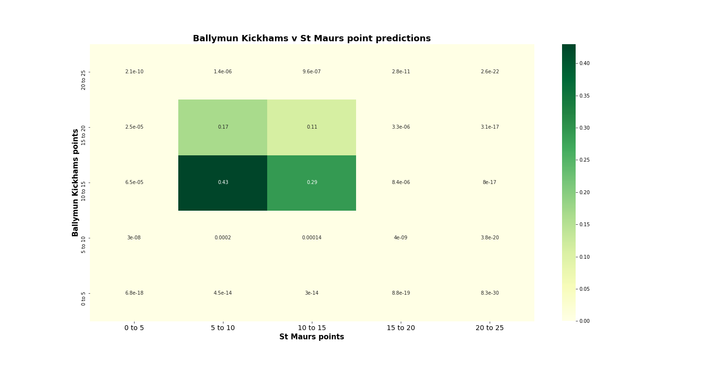
Plotting the output of this function shows us that the point scoreline with the highest probability is Ballymun scoring between 10-15 points and Maurs scoring between 5-10.

Simulating goals

Since we are not dealing with a continuous distribution, calculating goal probabilities is actually a lot more straight forward. We simply calculate the expected goals for a team against a given opponent (as described in section 5), and plug this value into the poisson formula from section 4 to iteratively calculate the probability of a team scoring 𝑥x goals in the match.

Similarly to before, we will create a function simulate_goals that will do this for us and we will plot the results on a heat map.

def simulate_goals(poisson_model, home_team, away_team, max_goals=5):
    # calculate home team expected goals using our poisson regression model
    home_team_expected_goals = poisson_model.predict(
        pd.DataFrame(data={'team': home_team, 'opponent': away_team, 'at_home':1},index=[1])
    )
    
    # calculate away team expected goals using the same model
    away_team_expected_goals = poisson_model.predict(
        pd.DataFrame(data={'team': away_team, 'opponent': home_team, 'at_home':0},index=[1])
    )
    
    # now loop through all possible goal combinations and determine the probability of that scoreline
    team_goals_prob = [
        [poisson.pmf(i, expected_goals) for i in range(0, max_goals+1)] for expected_goals in [
            home_team_expected_goals, away_team_expected_goals
        ]
    ]
    
    return (np.outer(np.array(team_goals_prob[0]), np.array(team_goals_prob[1])))
 
 
 
     
home_team = "Ballymun Kickhams"
away_team = "St Maurs"
 
match_score_probabilities = simulate_goals(poisson_model, home_team, away_team)

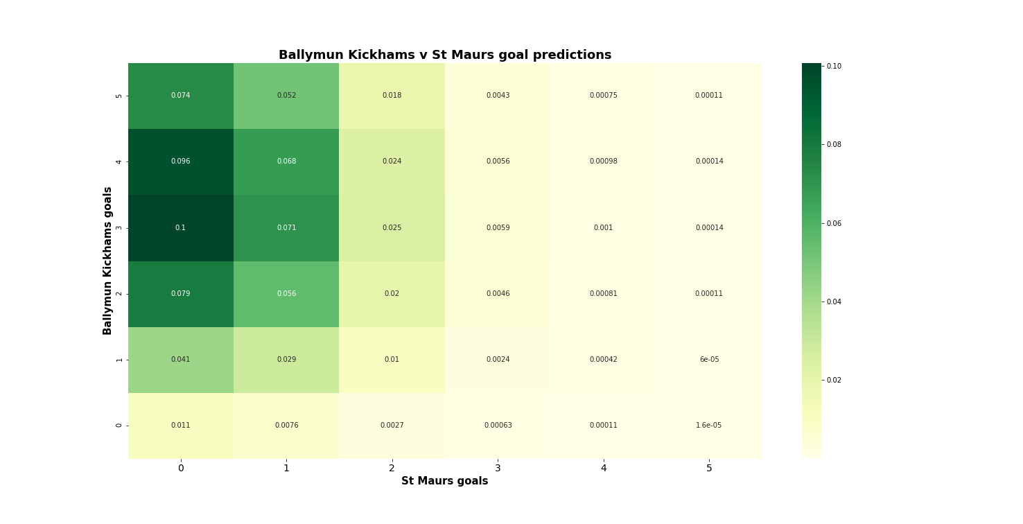
When we take a look at the output plotted below we can see that Ballymun are potentially in for a big day when they play Maurs, with a relatively high probability of them scoring 2 or more goals while conceding none!

Simulate full match

For the purposes of this section, let us assume that scoring a point and scoring a goal are independant events (i.e. scoring a point has no influence on you scoring a goal and vice versa).

With this assumption we can calculate the probability of a team scoring 𝑥 goals and 𝑦 points in a game as:

With this in mind, we can simulate all possible outcomes for a match between two teams and calculate the probability of either team winning. We will do this by:

1. Determine the expected goals and points for each team in the match

2. Iterate over all possible goal and point combinations (within reason) and determine the probabilities of those for both teams

3. Convert these goal and point combinations into total points (i.e. total points = 3*goals + points)

4. For each total point possibility determine the probability of the team achieving that total (e.g. the probability of scoring 3 total points is the probability of scoring 1 goal and 0 points + the probability of scoring 0 goals and 3 points)

5. Create an NxN probability matrix of all possible outcomes

6. Determine probability of home team winning by summing everything below the diagonal

7. Determine the probability of a draw by summing the diagonal

8. Determine probability of away team winning by summing everything above the diagonal.

We can wrap the above up in a function which will take two team names and determine the probability of either team winning the match.

def get_team_expected_goals(team, opponent, at_home, goals_model=poisson_model):
    
    team_expected_goals = goals_model.predict(
        pd.DataFrame(data={'team': team, 'opponent': away_team, 'at_home':at_home},index=[0])
    ).iloc[0]
    
    return team_expected_goals
 
 
 
def get_team_expected_points(team, opponent, at_home, points_model=normal_model):
    
    # calculate home team expected points and standard error using the normal model
    team_expected_points = points_model.predict(
        pd.DataFrame(data={'team': team, 'opponent': opponent, 'at_home': at_home},index=[1])
    ).iloc[0]
    team_se = points_model.get_prediction(
        pd.DataFrame(data={'team': team, 'opponent': opponent, 'at_home': at_home},index=[1])
    ).se_mean[0]
    
    return (team_expected_points, team_se)
 
 
 
def simulate_match(home_team, away_team, max_goals=10, max_points=35):
    
    # Step 1:
    home_team_expected_goals = get_team_expected_goals(home_team, away_team, 1)
    home_team_expected_points = get_team_expected_points(home_team, away_team, 1)
    home_team_expectation = {
        'team': home_team, 'expected_goals': home_team_expected_goals, 'expected_points': home_team_expected_points
    }
    
    away_team_expected_goals = get_team_expected_goals(away_team, home_team, 0)
    away_team_expected_points = get_team_expected_points(away_team, home_team, 0)
    away_team_expectation = {
        'team': away_team, 'expected_goals': away_team_expected_goals, 'expected_points': away_team_expected_points
    }    
 
    # Step 2:
    # loop through all goal and point combinations and determne probability and winner
    simulation_df = pd.DataFrame()
    index=0
    for expectation in [home_team_expectation, away_team_expectation]:
        for goal in range(max_goals+1):
            goal_prob = poisson.pmf(goal, expectation['expected_goals'])
            for point in range(max_points+1):
                # remember we cant predict exact numbers usng 
                probabiltity_more_than = norm(expectation['expected_points'][0], expectation['expected_points'][1]).cdf(point-0.5)
                probabiltity_less_than = norm(expectation['expected_points'][0], expectation['expected_points'][1]).cdf(point+0.5)
                point_prob = probabiltity_less_than - probabiltity_more_than
                
                scoreline_dict = {
                    'team': expectation['team'],
                    'goal': goal,
                    'goal_prob': goal_prob,
                    'point': point,
                    'point_prob': point_prob,
                    'total_score': (goal*3) + point,
                    'total_prob': goal_prob * point_prob
                }
                
                simulation_df = simulation_df.append(pd.DataFrame(scoreline_dict, index=[index]))
                index+=1
    # Step 3:           
    # now lets aggregate up to team and total score level
    # since a team can achieve a total score multiple ways, the probability of achieveing that score
    # is the sum of the probabilities of those ways
    simulation_df = simulation_df.groupby(['team', 'total_score'])['total_prob'].sum().reset_index()
    
    # Step 4
    # now lets create an n x n matrix of score probabilities
    home_team_probs = np.array(
       simulation_df.loc[simulation_df['team']==home_team].sort_values(by='total_score')['total_prob']
    )
 
    away_team_probs = np.array(
        simulation_df.loc[simulation_df['team']==away_team].sort_values(by='total_score')['total_prob']
    )
    
    # Step 5
    # here is the nxn
    result_probs = np.outer(home_team_probs, away_team_probs)
    # now we can get win probabilities by looking:
    #     - anything left of diagonal implies home team win
    #     - along diagonal ipmplies draw
    #     - right of diagonal implies away team win
    
    # Step 6, 7, & 8
    return {
        'home_team': home_team,
        'away_team': away_team,
        'home_team_win_prob': np.sum(np.tril(result_probs, -1)),
        'draw_prob': np.sum(np.diag(result_probs)),
        'away_team_win_prob': np.sum(np.triu(result_probs, 1))
    }

Running the function defined above across a number of matches, as demonstrated below, will give us the probability each team has of winning based on all possible outcomes.

matches = [
    ("Ballymun Kickhams", "Skerries Harps"),
    ("St Judes", "Kilmacud Crokes"),
    ("Ballinteer St Johns", "St Vincents"),
    ("Fingallians", "Ballyboden St Endas"),
    ("St Maurs", "St Oliver Plunketts ER"),
]
 
for match in matches:
    sim_result = simulate_match(match[0], match[1])
    print(f"{match[0]} v {match[1]}")
    print(f"Probability of {sim_result['home_team']} win: {round(sim_result['home_team_win_prob'], 2)}")
    print(f"Probability of draw: {round(sim_result['draw_prob'], 2)}")
    print(f"Probability of {sim_result['away_team']} win: {round(sim_result['away_team_win_prob'], 2)}\n\n")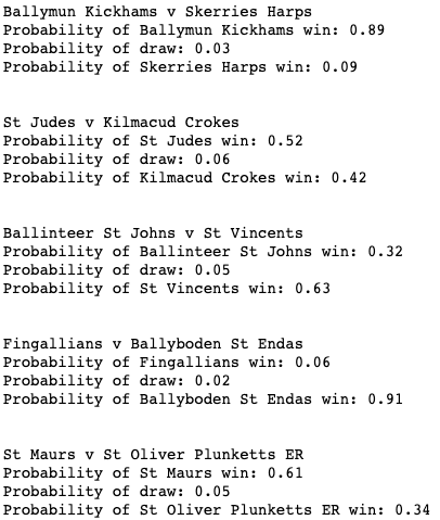

Closing thoughts

While this tutorial focused on the domain of Gaelic football, the methodology described can be applied across a number of sports and I would encourage readers to build their own models for other sports. For example, you could build a poisson model to simulate soccer matches, a normal model to simulate basketball matches, or if you want more practice combining both models you could scrape some hurling data and build a model for hurling.

If the data is available for your chosen sport, I would encourage you to explore the idea of including additional predictors in your models such as average possession per game or number of passes per game for each team as these could improve model results. If you are focusing on this dataset, you may try excluding the at_home variable (which isn’t statistically significant) and see how different the predictions are.