Deep learning: Activation functions

Published 2021-07-23

In this blog post I will be discussing activation functions for deep neural networks. I will begin by explaining what an activation function is and how they carry information through the network before taking a closer look at some of the more commonly used activation functions, and when they are best deployed.

What is an activation function?

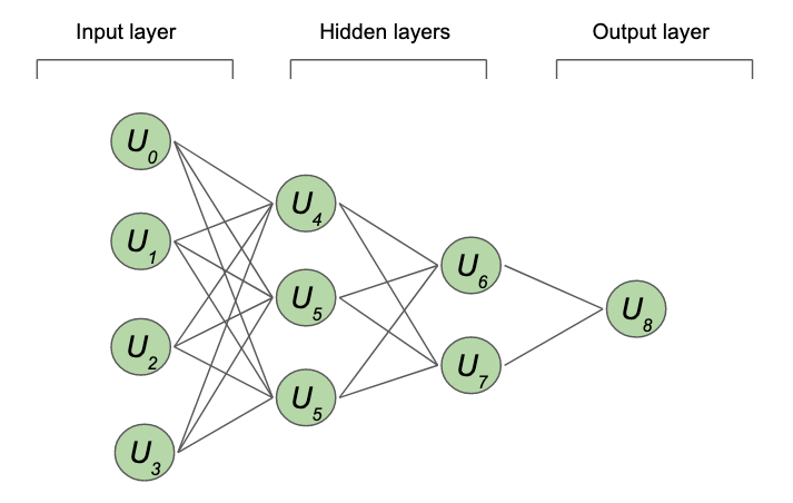
In a neural network comprised of N neurons (illustrated with a U in figure 1), the activation functions of the network determine what information is passed from one node to the next. These activation functions are typically scaler functions, meaning they take in multiple values (e.g. outputs from the preceding layer) but output a scaler, which is what gets passed to the next layer.

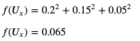
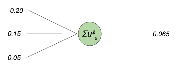
To get a better understanding of how activation functions work, lets zoom in on one particular neuron in a sample network. Figure 2 illustrates a sample neuron 𝑈𝑥, with three inputs (from the previous layer) of 0.2, 0.15, and 0.05. In this example, let us assume that our node 𝑈𝑥 has an activation function of f(x) = Σx^2. This means that the output of our layer Ux will be:

Although activation functions operate on each neuron in the network, we typically define activation functions on a layer by layer basis, meaning that all neurons in the same layer will have the same activation function.

A summary of the most popular activation functions

Now that we have a bit of an understanding around what activation functions are, in this section I will summarise some of the most commonly used activation functions and describe when and where they are best deployed.

Linear

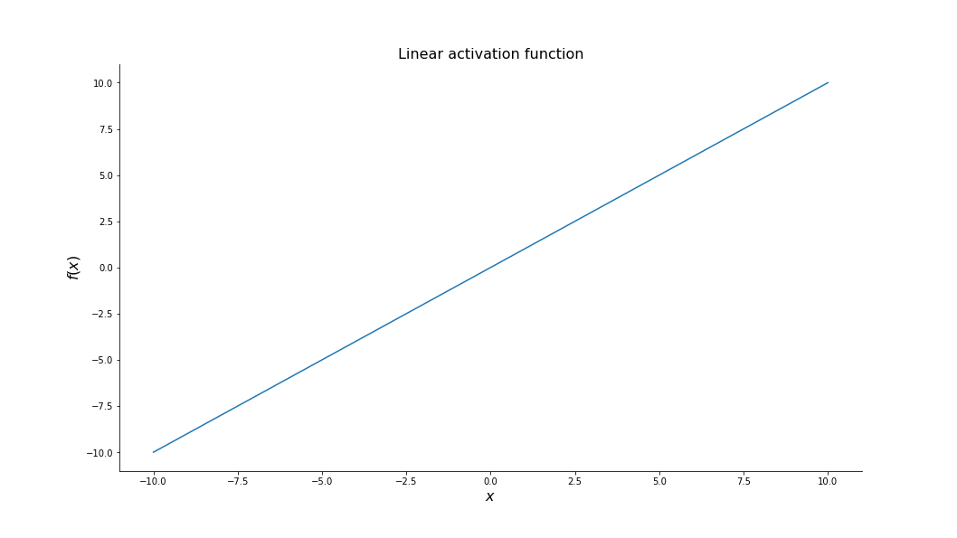
The linear activation function (illustrated in figure 3), is the most straightforward of all the functions covered in this blog post as it is simply the identity function (f(x) = x). From a practical point of view, this means that each neuron with a linear activation function allows it’s input signal to pass through unchanged.

With this in mind, linear activation functions are only really used in the input layer of a neural network.

Sigmoid

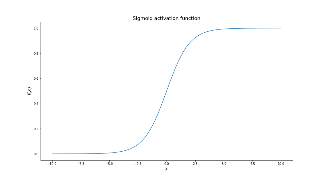
The sigmoid activation function, often called the logit function (defined below) is a commonly used function in machine learning which you may recognise from logistic regression. This function will always output a value between 0 and 1. It is because of this that the sigmoid activation function is commonly deployed within the hidden layers deep learning architectures as the fact that the output will always lie between 0 and 1 means that the network will be less impacted by extreme, or anomalous input values that the model hasn’t seen before during the feed forward process.

For example a linear activation function would output a value of 1 million if it somehow received an input of 1 million. This output could have knock on effects throughout the network and lead to an inaccurate output. The sigmoid activation function would handle this extreme input by outputting a value close to 1, and this will be far less likely to have an extreme impact on the models output.

Since the sigmoid activation function always outputs a value between 0 and 1, we can also use the activation function in the final layer of any binary classification task and use this output as the probability that the input data belongs to the binary class (i.e. if the output is greater than 0.5, then it is classified as belonging to whatever class you are trying to predict).

Tanh

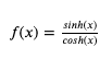
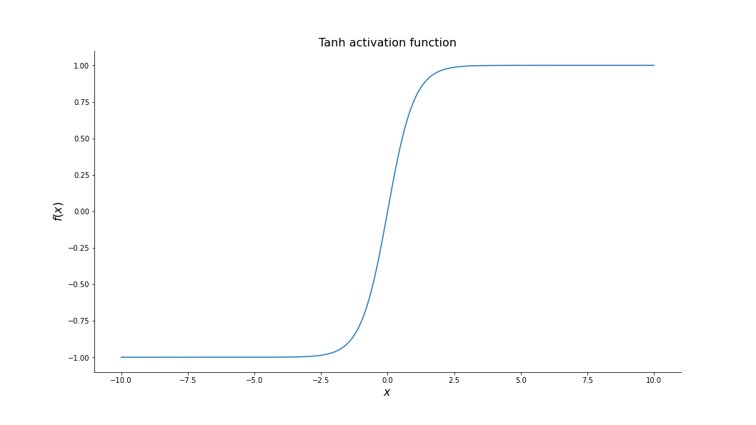
The tanh function (defined below) behaves very similarly to the sigmoid function discussed above, except for the fact that the output value will always fall within the range (-1, 1), rather than (0, 1).

The main difference between the sigmoid and tanh activation functions is that the tanh function handles negative values a lot better as larger negative values will be mapped to strongly towards -1 (and vice versa with larger positive values). For this reason, the tanh activation function is most commonly deployed within the hidden layers of deep learning architectures when your input data may contain negative values.

ReLU

The rectified linear unit activation function, commonly referred to as the ReLU activation function is an activation function which behaves similarly to the linear function when the output is greater than 0, but outputs 0 when the input is < 0. This may seem like a less accurate version of the linear function, however since the gradient the ReLU function is either 0 or a constant, it reduces the likelihood of the network experiencing a vanishing/exploding gradient.

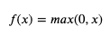
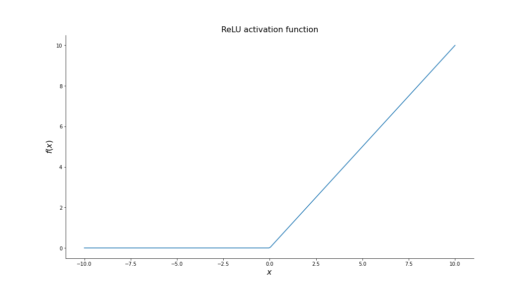
The vanishing/exploding gradient problem is a challenge faced by deep learning models when updating their weights between each epoch. Essentially what happens is that as the error on the training set is back propagated through the network, each weight (the lines in figure 1) is updated based the partial derivative of the error with respect to that weight, however if the gradients of these weights are too large or too small the model’s training process could be negatively impacted. In the case where the gradients get too large, the network will be unable to determine the loss of the model (you will get a NaN loss) and the training process will terminate. And in the case where the gradients are too small, the model will struggle to pick up on fine grained differences between each input and as a result the model may be less accurate than it could be.

It is because of the ReLUs ability to deal with the vanishing/exploding gradient problem (compared to other activation functions such a sigmoid and tanh) that many consider it to be the current state of the art. The ReLU activation function when deployed, should be used within the hidden layers of your architecture.

Leaky ReLU

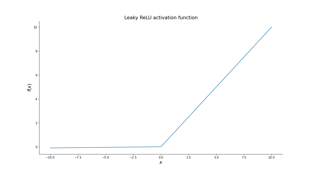
The Leaky ReLU function behaves extremely similar to the ReLU function defined above except instead of the output of this function being 0 for values less than 0, the function (defined below) will output a small negative slope.

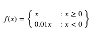
While the leaky ReLU function does not handle the exploding/vanishing gradient as well as the standard ReLU activation function, the leaky ReLU activation function is commonly used for tasks which may suffer from sparse gradients in an attempt to give the model some more signal to work for with. A common use for the leaky ReLU activation function is in training of general adversial networks (GANs).

Softmax

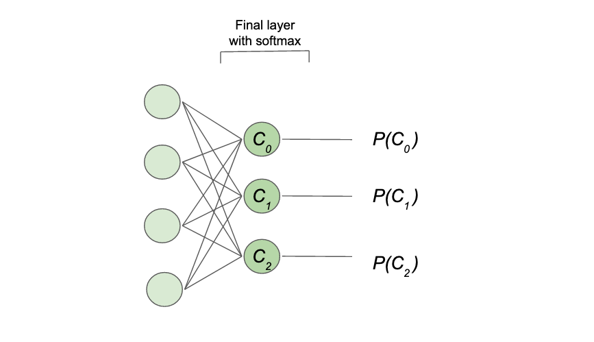
The softmax activation function can be thought of as a generalisation of the sigmoid function across multiple dimensions and is typically only used in the output layer of a (non-binary) categorical classifier. In other words, if we are building a neural network to classify data into N categories, this is the activation function we will use in the final layer.

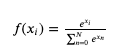
Essentially this activation function works by taking the exponential of each output (e.g. category) and divides it by the sum of the exponential for all the categories (see equation above). What we are left with after this (illustrated in figure 8) is a probability distribution that the input data belongs to each class. We can then simply take the class with the largest probability and say our model predicted the input data to belong to this class.