Building a simple expected pass completion (xP) model using Keras
Published 2021-07-03
In this blog post I will be going through how we can train a deep learning model, using passing event data from the StatsBomb open data repository to develop a simple expected pass completion model.
I will begin by stepping through the data preparation process before getting stuck into the modelling side of things and discussing some of the short comings of this particular model and how it could with improved. From here, I will go through two simple use cases for the model’s output.
As always, I have made a jupyter notebook with all the code used as part of this blog post available from my GitHub repository.
Data preparation
Acquiring the dataset
As mentioned in the introduction, the dataset we will use for this tutorial will be the StatsBomb open event dataset. This dataset contains match and event (passes, shots, etc.) data (in JSON) for 844 matches between 16-08-2003 and 23-02-2020.
Getting access to the data is very straightforward, you can simply clone the StatsBomb open data repository to your local machine.
Once downloaded, you will see all the data we need within the data subdirectory. You will also find a guide on how each of the match and event files relate to each other on the homepage of the repository.
Building a dataframe of pass events
Once the dataset has been downloaded, the next step will be to iterate through each file within the /events subdirectory and extract what we deem to be the required information about each passing event. The model developed as part of this tutorial will focus on the following datapoints:
-
match_id: Numeric identifier to track the match the passing event occurred in (just pulled for tracking/debugging) -
event_id: UUID identifier for the event (just pulled for tracking/debugging) -
passing_team: The name of the team who passed the ball (Can be used to filter the data later once the model is trained) -
passing_player: The name of the player who passed the ball (Can be used to filter the data later once the model is trained) -
recipient_name: The name of the player that the pass was intended for (Can be used to filter the data later once the model is trained) -
passing_player_x_location: The player who is passing the balls x-axis position on the pitch (see the StatsBomb documentation appendix for more info on this) -
passing_player_y_location: The player who is passing the balls y-axis position on the pitch -
pass_end_location_x: The x-axis location on the pitch where the ball finished up -
pass_end_location_y: The y-axis location on the pitch where the ball finished up -
pass_height_category: Categorisation of how high the pass was, one of ground_pass, low_pass, or high_pass(further information on how these are categorised can be found in the statsbomb documentation) -
body_part: What part of the body the player used when attempting the pass (left foot, right foot, head, etc.) -
outcome: The result of the pass, one of “Incomplete”, “Injury Clearance”, “Out”, “Pass offside”, “Unknown” or None(implying complete).
Using the code segment below we can extract all of this information from the source data by loading each JSON object into python as a dictionary before using the .get() method to pull the required fields and store them in a list of dictionaries which we can very easily convert to a pandas dataframe object at the end of the loop.
event_data_dir = 'open-data/data/events'
pass_data = []

# iterate through each file in the events data directory and pull each event if it is a passing event
for filename in tqdm(os.listdir(event_data_dir)):
    if filename.endswith(".json"):
        with open(os.path.join(event_data_dir, filename)) as json_file:
            match_id = int(filename[:-5])
            data = json.load(json_file)
            for event in data:
                if event.get('type', {}).get('name', None) == 'Pass':
                    pass_data.append(
                        {
                            'match_id': match_id,
                            'event_id': event['id'],
                            'passing_team': event.get('possession_team', {}).get('name', None),
                            'recipient_name': event.get('pass', {}).get('recipient', {}).get('name', None),
                            'passing_player': event.get('player', {}).get('name', None),
                            'passing_player_x_location': event['location'][0],
                            'passing_player_y_location': event['location'][1],
                            'pass_end_location_x': event.get('pass', {})['end_location'][0],
                            'pass_end_location_y': event.get('pass', {})['end_location'][1],
                            'pass_height_category': event.get('pass', {}).get('height', {}).get('name', None),
                            'body_part': event.get('pass', {}).get('body_part', {}).get('name', None),
                            'outcome': event.get('pass', {}).get('outcome', {}).get('name', None)
                        }
                    )
# Note that "None" outcome means complete
pass_df = pd.DataFrame(pass_data)
pass_df.head()
Convert our dataframe into something we can use for modelling
Before we get stuck into the modelling side of things we will have to transform our dataset into something our model will be able to interpret. This will involve 4 steps:
-Remove passing events with invalid outcomes: This involves dropping any rows which have an outcome of “Injury Clearance”, “Pass offside”, or “Unknown”. The reason for dropping these rows is that these are either not real passes (Injury clearance are just people putting the ball out of play, and offside passes technically don’t happen as far as the game is concerned) or the outcome is unknown.
-
One hot encode categorical columns: This is a common practice in any modelling task and involves us turning our categorical variables (
pass_height_categoryandbody_part) into a series of N binary columns, each column representing a value which the categorical variables can take (see here for more information). In our example we would create binary columns for “left foot”, “right foot”, “low pass”, “high pass”, etc. -
Created a binary column to say if the pass was completed or not: This step involves us creating the target column for our model. This will simple be a binary column called completed which will take the value of 1 if completed and 0 if not.
-
Drop columns the model wont need to analyse: This step involves removing columns that provide little to no information about the pass (such as
match_id,event_id,passing_team,recipient_name) or columns which simply contain too many distinct categorical values to model (such aspassing_player)
Thankfully for us, pandas makes the 4 transformations listed above incredibly straightforward, as demonstrated below:
# Step 1: remove pass events we don't want
modelling_df = pass_df.loc[
    ~pass_df['outcome'].isin(['Injury Clearance', 'Pass Offside', 'Unknown'])
]

# Step 2: create one hot variables
# pass height and body part
one_hot_pass_height_variables = pd.get_dummies(modelling_df['pass_height_category'])
one_hot_body_part_variables = pd.get_dummies(modelling_df['body_part'])

# tidies up naming befor appending row wise
one_hot_pass_height_variables.columns = [
    col.lower().replace(' ', '_') for col in one_hot_pass_height_variables.columns
]
one_hot_body_part_variables.columns = [
    col.lower().replace(' ', '_') for col in one_hot_body_part_variables.columns
]

modelling_df = pd.concat([modelling_df, one_hot_pass_height_variables], axis=1)
modelling_df = pd.concat([modelling_df, one_hot_body_part_variables], axis=1)

# Step 3: create binary pass complete column
modelling_df['completed'] = 0
modelling_df.loc[modelling_df['outcome'].isna(), 'completed'] = 1

# Step 4: finally filter down to the columns we want
modelling_cols = (
    [
        'passing_player_x_location',
        'passing_player_y_location',
        'pass_end_location_x',
        'pass_end_location_y'
    ] +
    list(one_hot_pass_height_variables.columns) +
    list(one_hot_body_part_variables.columns) +
    ['completed']
)

modelling_df = modelling_df[modelling_cols]
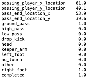
This creates one row per passing event which looks like the following sample:
Train test split
Now that we have a modelling dataframe ready to go, our next task is to split our dataset into 3 partitions. One training partition that our model will be trained on, a validation partition which our model will use to assess it’s own performance during training, and a testing partition which we will use to assess the models performance ourselves once training is complete.
To do this we can use sklearn’s train_test_split function to split the dataset into 80% training, 15% testing, and 5% validation as illustrated below.
# Here X represents our predictors (location, height, body part) and y represents our target (completed)
X = modelling_df.iloc[:, :-1]
y = modelling_df.iloc[:, -1]

X_train, X_test, y_train, y_test = train_test_split(
    X, y, test_size=0.8, random_state=123, stratify=y
)


X_test, X_val, y_test, y_val = train_test_split(
    X_test, y_test, test_size=0.25, random_state=123, stratify=y_test
)
Oversample minority class
The final step (thankfully) before we get stuck into the modelling side of things requires us to balance out the training dataset to ensure our model is seeing the same number of completed and incompleted passes. Without performing this step, our model could figure out that it is better off ignoring any of the underlying data and that it can achieve a high accuracy score by predicting that every pass is complete.
To balance out our dateset, we will sample incomplete passes from our training set and very slightly modify the x and y coordinates of the passing player and outcome (to ensure the model is seeing slightly varied data) before appending it to our training set. This process will be repeated until our training dataset contains the same number of complete and incomplete passes.
negative_samples = y_train.value_counts()[0]
positive_samples = y_train.value_counts()[1]
current_negative_samples = pd.concat([X_train, y_train], axis=1)
current_negative_samples = current_negative_samples.loc[current_negative_samples['completed'] == 0].iloc[:, :-1]
additional_negative_samples = []
y_vals = []

while negative_samples < positive_samples:
    sample_for_smote = current_negative_samples.sample().to_dict(orient='records')[0]
    smote_player_x_loc = sample_for_smote['passing_player_x_location'] + random.uniform(-4, 4)
    # do a small bit of smote
    sample_for_smote['passing_player_x_location'] = (
        sample_for_smote['passing_player_x_location'] + random.uniform(-4, 4)
    )
    sample_for_smote['passing_player_y_location'] = (
        sample_for_smote['passing_player_y_location'] + random.uniform(-4, 4)
    )
    sample_for_smote['pass_end_location_x'] = (
        sample_for_smote['pass_end_location_x'] + random.uniform(-4, 4)
    )
    sample_for_smote['pass_end_location_y'] = (
        sample_for_smote['pass_end_location_y'] + random.uniform(-4, 4)
    )
    additional_negative_samples.append(sample_for_smote)
    y_vals.append(0)
    negative_samples += 1

X_train = pd.concat([X_train, pd.DataFrame(additional_negative_samples)]).reset_index(drop=True)
y_train = pd.concat([y_train, pd.Series(y_vals)]).reset_index(drop=True)
Modelling
Train our model
Once the data preparation is complete, the modelling process is relatively straightforward. We will begin by creating a simple 4 layer dense neural network as demonstrated by the below function:
def create_model():
    model = Sequential()

    model.add(BatchNormalization())
    model.add(Dense(128))
    model.add(ReLU())
    model.add(Dropout(0.5))

    model.add(Dense(64))
    model.add(ReLU())
    model.add(Dropout(0.5))

    model.add(Dense(8))
    model.add(ReLU())
    model.add(Dropout(0.5))

    model.add(Dense(1, activation='sigmoid'))

    optimizer = Adam(learning_rate=0.001)

    model.compile(optimizer=optimizer, loss='binary_crossentropy', metrics=['accuracy'])

    return model
From here, we will create our model using this function before defining a few Keras callbacks which will prevent our models from overfitting during training and will handle any learning rate reductions which may be required if our model gets stuck in any local minima.
Once these are defined, we can pass our modelling dataframe (in the form of a numpy array) into the model and start training!
model = create_model()

# some model callbacks to improve results on monitor training
save_best_model = ModelCheckpoint("pass_model.hdf5",monitor="val_loss")
terminate_on_nan = TerminateOnNaN()
csv_logger = CSVLogger('training.log')
dynamic_lr = ReduceLROnPlateau(
    monitor='val_loss', factor=0.1, patience=15, verbose=0, mode='auto', cooldown=0, min_lr=0
)
stop_early = EarlyStopping(
    monitor='val_loss', min_delta=0, patience=25, verbose=0, mode='auto'
)

# Here is where the model actually trains
model_history = model.fit(
    np.array(X_train).astype('float32'),
    np.array(y_train).astype('float32'),
    batch_size=128,
    epochs=100,
    verbose = 1,
    callbacks=[save_best_model, terminate_on_nan, dynamic_lr, stop_early, csv_logger],
    validation_data=(
        np.array(X_val).astype('float32'),
        np.array(y_val).astype('float32')
    ),
    shuffle=True
)
Assess results
Once our model is finished training we can assess it’s performance on the testing set. We will do this using sklearn’s classification_report function on the actual versus predicted values from the model on our testing set.
# load the model
model = load_model("pass_model.hdf5")

y_pred = model.predict(np.array(X_test))
y_prob = y_pred
y_pred = y_pred > 0.5
print(classification_report(y_test, y_pred))
precision recall f1-score support
0 0.52 0.85 0.64 106880
1 0.95 0.80 0.87 416568
accuracy 0.81 523448
macro avg 0.74 0.82 0.76 523448
weighted avg 0.86 0.81 0.82 523448When we take a look at the outputs above, we can see that despite the models decent performance on predicting completed passes, the model did really struggle at identifying incompleted passes. Since we are just looking to develop a simple or baseline xP model in this tutorial, it’s not the end of the world but obviously if we were looking to use this model in production, we would have to look at improving it.
An easy way I would say this model could be improved is by acquiring additional player position data. Right now our model only knows the position of the passing player on the pitch and has no awareness of where the player they are trying to pass to is positioned, if they are being marked, and how many opponents stand between the passing player and the ball’s end position. I would wager that having access to this sort of data would significantly increase the accuracy of the model. In addition to this data, further refinement on the network itself could eeek out an extra few % in accuracy at the end.
Using the outputs of the model
Now that we have a model that can take a set of inputs data about a pass and predict how likely it thinks it will be that the pass is completed we can start playing around with the output.
Plotting pass probabilities
One simple thing we can do is take a set of passes and plot them on a map with their expected pass completion probability next to them as demonstrated below
import matplotlib.pyplot as plt
from mplsoccer import Pitch

model = load_model("pass_model.hdf5")
samples = modelling_df.sample(8, random_state=64).reset_index(drop=True)
samples['model_prob_success'] = model.predict(np.array(samples.iloc[:, :-1])).tolist()
pitch = Pitch(pitch_color='grass', line_color='white', stripe=True)
fig, ax = pitch.draw()

fig.set_size_inches(18, 11)
for index, row in samples.iterrows():
    player_x =  row['passing_player_x_location']
    player_y = row['passing_player_y_location']
    ball_end_x = row['pass_end_location_x']
    ball_end_y = row['pass_end_location_y']
    model_prob_success = round(row['model_prob_success'][0]*100, 2)
    colour = 'white' if row['ground_pass'] == 1 else '#ffffb3' if row['low_pass'] == 1 else 'black'
    label = 'Ground pass' if row['ground_pass'] == 1 else 'Low pass' if row['low_pass'] == 1 else 'High pass'
    completed = 1 if row['completed'] ==  1 else 0
    ax.arrow(
        x=player_x,
        y=player_y,
        dx=ball_end_x - player_x,
        dy=ball_end_y - player_y,
        width=1,
        color=colour,
        label=label,
    )
    ax.annotate(
        f"{model_prob_success}%",
        xy=(player_x - 10, player_y + 1),
        color=colour,
        size=17,
        weight='bold'
    )
ax.set_title(
    "Probability of pass completion using model on 7 samples from our modelling dataframe\n"
    "where team in possession is attacking from left to right",
    size=18,
    weight='bold'
)
handles, labels = plt.gca().get_legend_handles_labels()
by_label = dict(zip(labels, handles))
ax.legend(by_label.values(), by_label.keys(), title="Pass height category", loc='upper left')
plt.gca().invert_yaxis()
fig.savefig(f"pass_probabilities.png", bbox_inches="tight")
plt.show()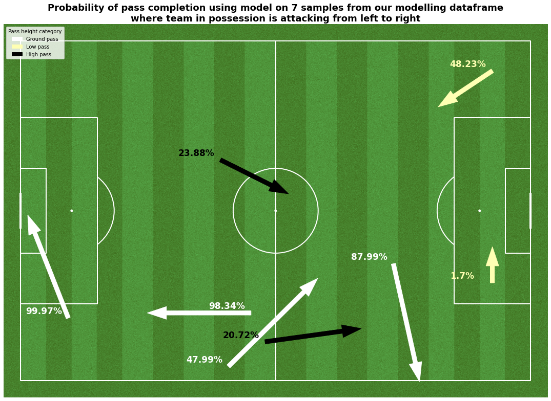
With access to the right data, a team could easily spin up a chart like this for each player to help them improve their performance when it comes to selecting the right pass.
Identifying who are the safest passers on the team
Another simple output one could create from this type of model is a ranking of players based on their mean pass completion probability, this could give managers an idea of which players on the team take the most chances, and which can be trusted to do the right thing on the ball.
Using the StatsBomb data, I was able to pull out every pass made by Arsenal’s invincibles team and rank the players in order of their mean expected pass completion.
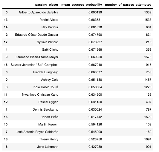
When we take a look at the output above, we can see that perhaps unsurprisingly the midfield pairing of Gilberto and Vieira are the safest passers of the ball, while the goalkeeper (who probably takes a lot of kickouts that are deemed risky) has the lowest mean expected completion rate. I was however very surprised to see the likes of Henry so low on this list, perhaps the advance positions he took up on the pitch, and the amount of attention he likely drew from defenders played into this.
Closing thoughts
In this blog post, I went through how we can use the StatsBomb open data repository to create a dataset of passes and use this data to train a simple deep learning network to predict the likelihood that the pass will be completed. While there are some shortcomings to the modelling approach detailed in this blog (primarily around the lack of player positional data taken into account), we showed how the outputs of this baseline model could be used to generate a couple of outputs which may be useful to a team who are looking to select the most reliable players on matchday, or help improve their players decision making through data visualisation.
I would encourage anyone to try build on top of the work done in this blog post by improving the model through additional data or fine tuning, or by creating more interesting visualisations with the outputs.
Once again, if you would like access to the source code for this blog post, you can find it my GitHub repository.