An introduction to linear programming in python
Published 2020-07-20
Table of Contents
In this blog post I will be discussing linear programming, a mathematical method used to determine the optimal solution to a linear equation subject to linear constraints. I will begin by introducing the idea of linear programming and what a typical linear programming problem looks like. From here I will work step by step through a simple profit maximisation problem using the PuLP python library.
If you would like a more interactive tutorial, I have created a jupyter notebook with a summarised version of this tutorial which you can download from my GitHub repository.
What is linear programming
Linear programming (LP) is a mathematical technique which allows us to determine the optimal values for the parameters of a linear function (known as an objective function) subject to some set of linear constraints. Depending on the nature of the problem the optimial solution will be defined as the solution which either minimises, or maximises the output of the objective function. Some common examples of LP problems include:
-
Maximising profit based on production constraints
-
Minimising distance to travel when delivering items
-
Maximising output from a factory based on time constraints
When formulated, a typical LP problem will look something like:
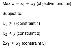
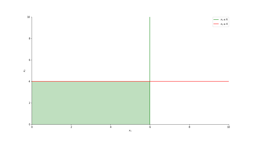
At this point it is understandable to wonder how we go about solving a problem in the format above and while there are many approaches one can take to solve a linear programming problem, the simplex method is probably the most popular approach. The simplex method works by identifying a feasible region for the problem which can be determined by plotting each of the problems constraints (see below). From here the algorithm walks along the edge of the feasible region, calculating the objective function at each step until the optimal solution is identified. The below example highlights the feasible region (in green) for an objective function with constraints x_1 <= 6 and x_2 <= 4.
Working example in Python
Of course when we implement LP in python using PuLP, we don’t have to worry about plotting the feasible region (although it can be helpful) as the library will handle this in the background. However oftentimes I find the hardest part of implementing LP is converting a problem worded in plain English into a LP formulation. With that in mind, in this section I will work through a simple LP problem, starting with the problem definition, converting it to a LP formulation, plotting the feasible region (optional), and solving using the PuLP library. hopefully this will give you a better understanding of the end to end process and will help when it comes to implementing LP on your own problems.
Define the problem
Consider the following problem:
“Computer Parts Ltd., a computer hardware manufacturer make two types of products, keyboards and mice. Each unit of keyboards takes 1.5 hours to make and yields €50 in profit. On the other hand each unit of mice takes 1 hour to make, but only yields €37 in profit.
Computer Parts Ltd. recently signed a contract with a local wholesaler guaranteeing the production of at least 7 units of keyboards per day and 8 units of mice. Also, in order to satisfy supply and demand, Computer Parts Ltd have agreed to produce no more than twice the number of mice as there are keyboards.
A recent contract with the workers union also states that Computer Parts Ltd. can have no more than 25 labour hours per day.
How many (whole) units of keyboards and mice should computer parts limited make per day in order to maximise their profits given their contractual obligations?”
Formulate the problem as a linear programming problem
In order to begin formulating this problem as a LP problem let us say that:

Since we want to maximise profits we can define the objective function z as:

Where 50 and 37 represent the profit made on the production of each item.
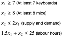
Finally we can formulate our constraints as defined in the original problem. This is typically the most difficult part of any LP problem so don’t be too worried if you make a mistake on this, you will get used to it. The constraints for our problem can be defined as follows:
Plot the feasible region (optional)
As mentioned above, formulating the constraints for an LP problem can sometimes be confusing and while it is not required when using a LP library like PuLP to solve a problem, I find it can be extremely useful to plot your problems constraints and identify the feasible region before solving to confirm your problem makes sense and that a feasible region exists.
As you can see below, we can do this by generating a set of values for x1 and x2 using numpy before plotting each of the constraint lines using matplotlib. Finally we can use the fill_between function to shade in the feasible region for our problem.
import numpy as np
import matplotlib.pyplot as plt

x_1 = np.linspace(0, 30, 1000)
x_2 = np.linspace(0, 30, 1000)

# plot
fig, ax = plt.subplots()
fig.set_size_inches(14.7, 8.27)

# draw constraints
plt.axvline(7, color='g', label=r'$x_1 \geq 7$') # constraint 1
plt.axhline(8, color='r', label=r'$x_2 \geq 8$') # constraint 2
plt.plot(x_1, (2*(x_1)), label=r'$x_2 \leq 2x_1$') # constraint 3
plt.plot(x_1, 25 - (1.5*x_1), label=r'$1.5x_1 + x_2 \leq 25$') # constraint 4


plt.xlim((0, 25))
plt.ylim((0, 30))
plt.xlabel(r'Number of keyboards ($x_1$)')
plt.ylabel(r'Number of mice ($x_2$)')

# fill in the fesaible region
plt.fill_between(x_1, np.minimum(25 - (1.5*x_1), (2*(x_1))), np.minimum(25 - (1.5*x_1), 8),
where=x_1 >= 7,
color='green', alpha=0.25)
plt.legend(bbox_to_anchor=(1, 1), loc=1, borderaxespad=0.)

# Hide the right and top spines
ax.spines['right'].set_visible(False)
ax.spines['top'].set_visible(False)
plt.show()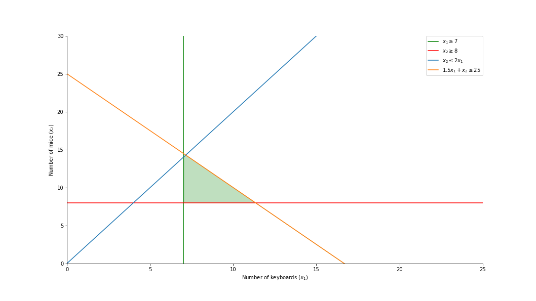
Looking at the output above we can see that a feasible region exists for our problem (shaded in green) and we would expect the optimal solution for our problem to be somewhere within the range 7-13 for x1 and 8-14 for x2.
Solve using PuLP
Once we have our problem se up, and we are confident that a solution exists, we are ready to solve our problem using PuLP. While there are other libraries out there for solving LP problems such as scipy and gekko, I find that the notation used in PuLP is way cleaner which makes it much easier to use.
The first steps when using PuLP are to create a model object which details the type of problem we are trying to solve (maximise in this case) and define the model variables (x1 and x2). It is worth noting that since we cannot produce half a unit of either product in our problem, we can set the variable type to integer. This will mean that our solution will be limited to whole numbers. You may notice that we can also set the lower bound for each of our variable values. This will eliminate the need to specify our first two constraints later on.
from pulp import LpMaximize, LpProblem, LpVariable

# first create a model object
model = LpProblem(name="computer_parts_problem", sense=LpMaximize)

# declare our variables
x_1 = LpVariable(name="x_1", lowBound=7, cat="Integer")
x_2 = LpVariable(name="x_2", lowBound=8, cat="Integer")
From here we can easily add the objective function to the model
# set the objective function for the model
model += (50 * x_1) + (37 * x_2)
Once the objective function is defined we can add our remaining two constraints to the model in a similar fashion. Once added, we can take a look at the model and confirm everything is OK.
# now we can add our constraints
model += (x_2 <= 2 * x_1, "supply_and_demand")
model += ((1.5 * x_1) + x_2 <= 25, "labour_hours")

# take a look at the model
print(model)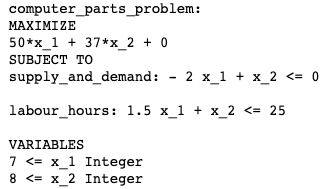
Once we are happy that we have correctly defined our objective function and it’s constraints, we can solve the problem using the solve() method. From here we can iterate through the model variables to print their optimal value before printing the optimal output from the objective function.
solution = model.solve()

for variable in model.variables():
    print(f"Optimal value for {variable.name} is {variable.value()}")

print(f"\nThis will yield a total profit of €{model.objective.value()}")
Doing this we can see that optimal solution for Computer Parts Ltd. is to produce 8 units of keyboards and 13 of mice for a profit of €881.
Closing thoughts
With the current hype surround machine learning and deep learning, problem solving methods such as linear programming are often overlooked. After reading this I hope you will agree that linear programming can be a very handy tool to have in our tool belt for solving many real world problems, and that libraries such as PuLP make it very easy to implement LP on our own problems.
Of course the major limitation on linear programming is that it is only capable of solving problems for which both the objective function and its constraints are linear. Oftentimes in the real world our problems will contain non-linear equations and are therefore unsolvable using linear programming. Thankfully for us however, we can solve these using non-linear programming (the original NLP).
In my next blogpost I will be discussing non-linear programming, the challenges posed by it, and how we can solve non-linear problems using python.
Exercises
If you would like some more practice solving linear programming problems expressed in plain English, I have included a couple of exercises below for you to have a go at.
-
A carpenter makes 2 products, tables and chairs. Each table can be sold for a profit of €30 while each chair for a profit of €10. The carpenter can afford to spend up to 40 hours per week working. It takes six hours to make a table and three hours to make a chair. Customer demand requires that he makes at least three times as many chairs as tables. Tables take up four times as much storage space as chairs and there is room for at most four tables each week. How much of each product should the carpenter produce to maximise their profit?
-
Tom wakes up to realise he has the day off work. This is great news as he recently bought a new game and he wants to spend some time playing it. Tom however has a charity run and cycle coming up in a few weeks which he needs to do some training for. He knows he will have to do at least 30Km of exercise today to ensure he is good to go for next week. He also knows that at least 7Km of this will have to be spent running and at least 15Km will be cycling. Since he doesn’t want to overdo it on the cycling he agrees that for each kilometre he cycles, he must also run at least 0.5 of a kilometre. If it takes tom 5 minutes to run a kilometre and 2 minutes to cycle the same distance, how should Tom structure his training to maximise the time he can spend playing his new game.