An introduction to graph neural networks: Classifying soccer player positions from passing networks
Published 2022-06-04
Table of Contents
In this blog post I will be discussing the idea of graph neural netowks and how we can use them to create a simple soccer player position classifier using the PyTorch Geometric framework on data from Italy's final 4 matches at Euro 2020.
This blog post is split into two sections. In section one I will give a brief overview of of graph neural networks, why they are needed, and how they work before getting stuck into the position classification example in section 2.
As always, I have provided the full code used for this tutorial in the my GitHub Repository!
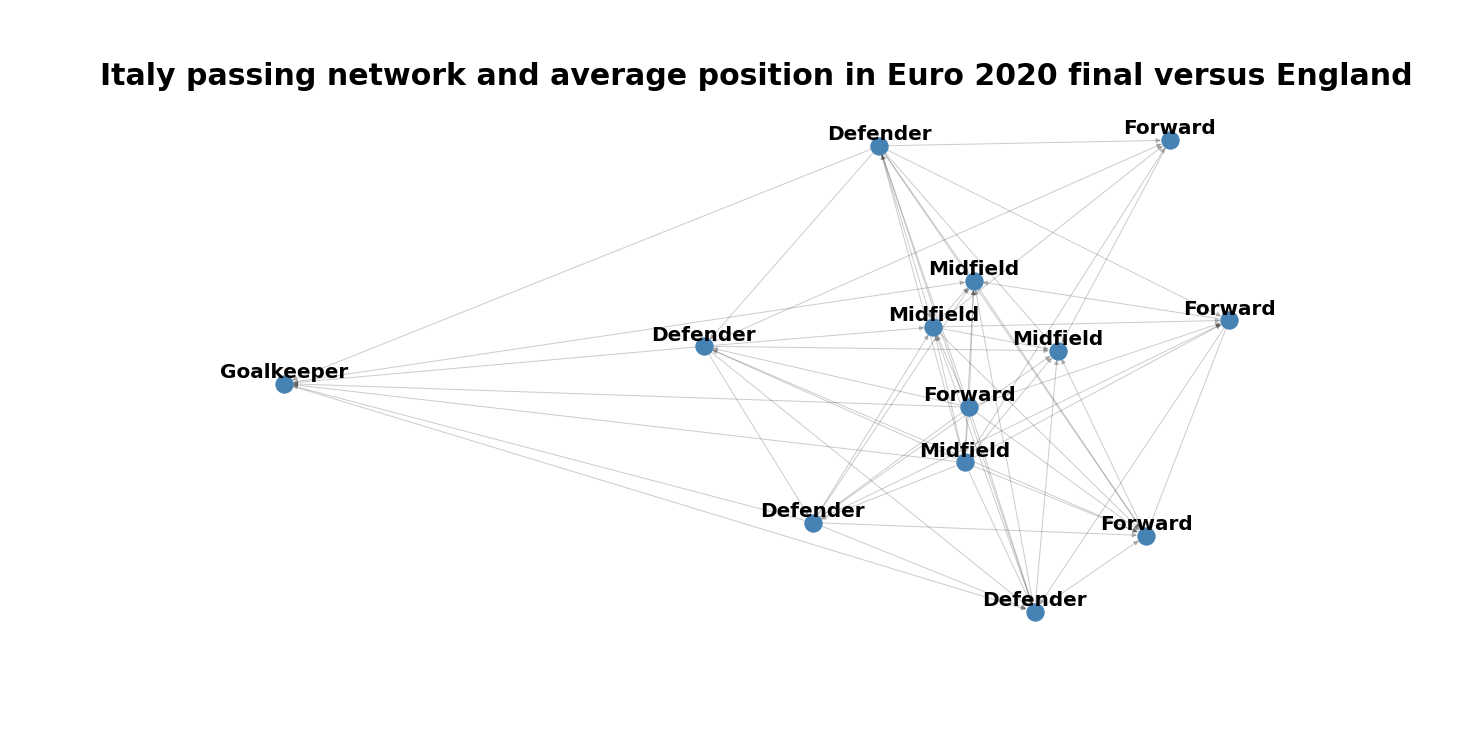
An introduction to graph neural networks
What are graph neural networks?
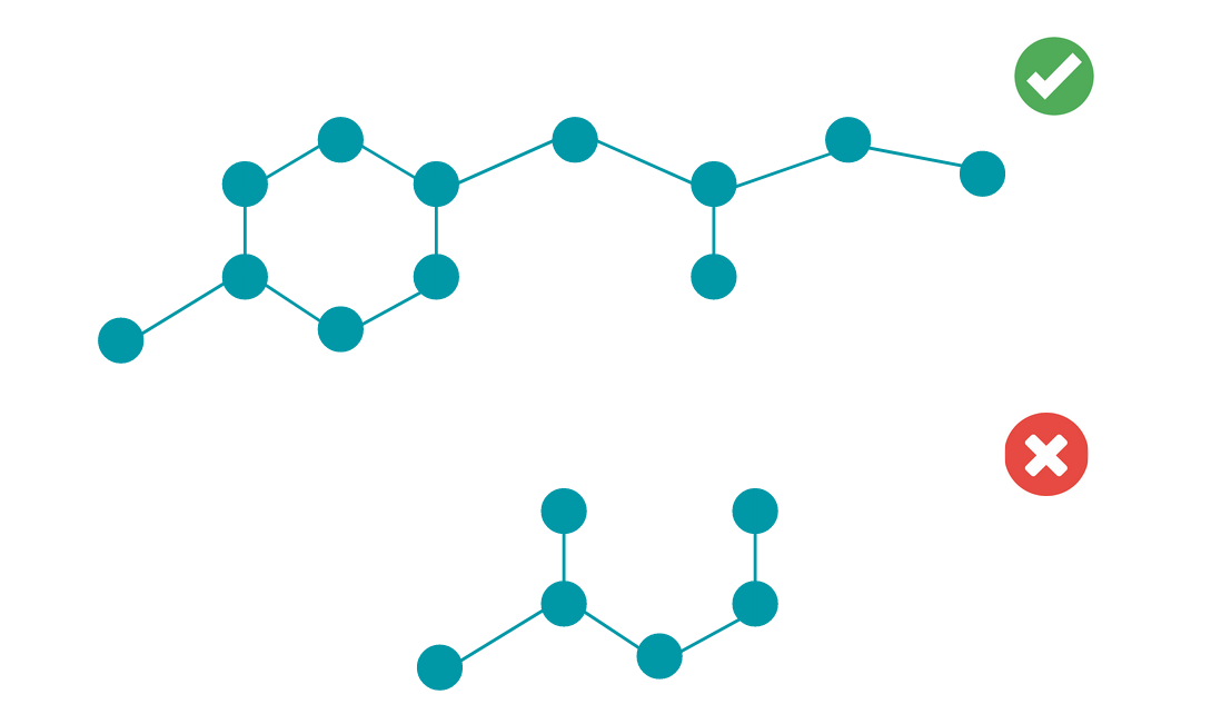
- Graph classification: In a graph classification task, the model will be used to predict some property of the graph as a whole. An example of this would be to classify whether a chemical compound is a protein or not based on it's molecular structure.
Graph neural networks (GNN) are a form of deep learning architecture which analyse data described by graphs. Typically the tasks which a GNN's are used for can be broken into 3 categories:
- Graph classification: In a graph classification task, the model will be used to predict some property of the graph as a whole. An example of this would be to classify whether a chemical compound is an protein or not based on it's molecular structure.
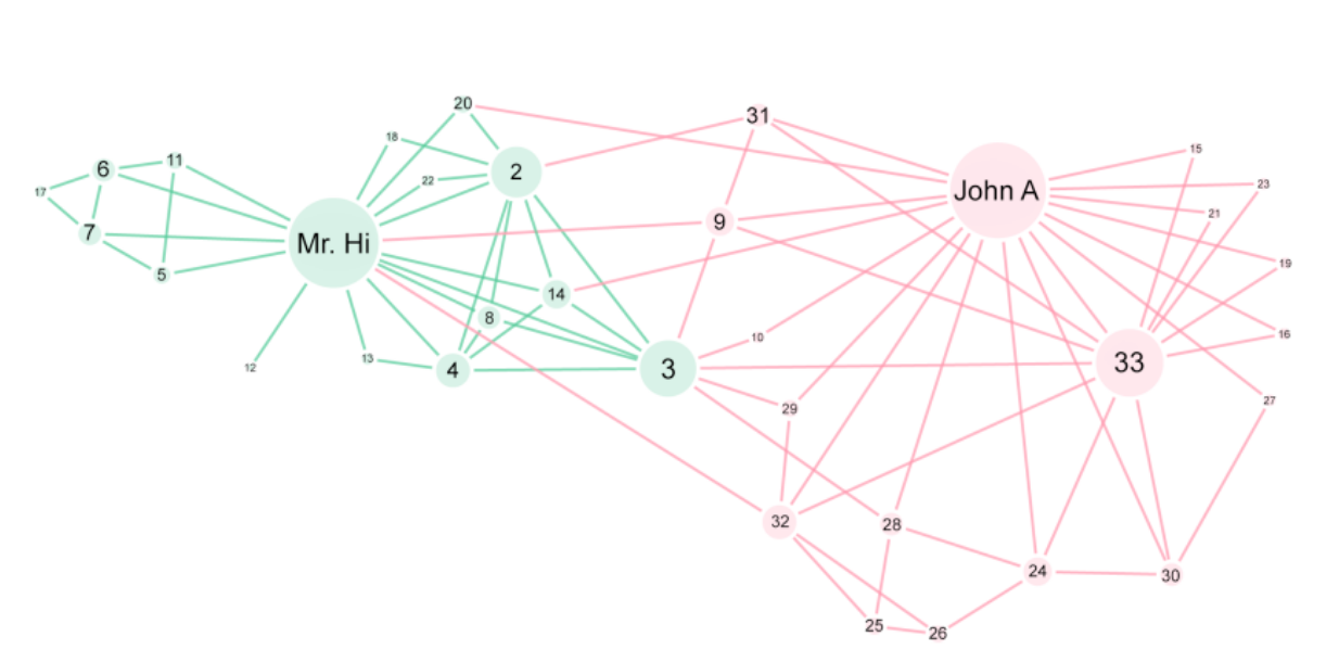
- Node classification: In a node classification task we are interested in classfying some property of each node within a graph. A classic example here is classifying each members loyalty to one of two instructors in the karate club dataset.
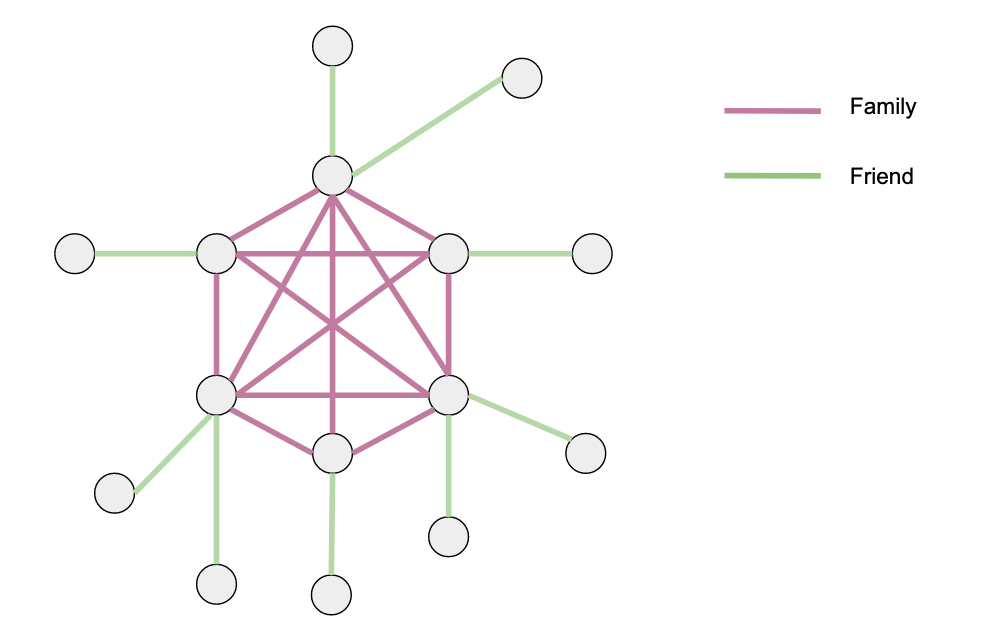
- Edge classification: Similar to node classification, edge classification problems involve classifying the relationship between nodes (the edges). An simple example here would be classifying edges in a social network into relationships such as friend, family, or even enemy.
Why do we need graph neural networks?
Those of you familiar with graphs, and who understand the concept of an adjacency matrix might be wondering why do we need a special type of deep learning network to analyse graphs, and why can't we just pass the graphs adjacency matrix through a traditional deep learning architecture?
This is reasonable question to ask, however there are 3 main reasons why we can't simply pass a graphs adjacency matrix through a traditional architecture:
-
Graphs in the "wild" can be very large with the number of nodes or edges in a graph being in the millions in some cases. Using an adjacency representation here causes big problems as since not all nodes are related, we can be left with extremely sparse, memory inefficient matrices which can cause problems when modelling.
-
Not all graphs are the same size. Similar to images, graphs can vary in size, however graphs are much harder to crop then images, so, if we wanted to limit the input size of the adjacency matrix for a model, we can't crop the graph and still maintain the information provided within the graph in the same way we would an image.
-
Finally, one graph can have many different adjacency matrices (see figure 4) and there is no way to guarentee that these different adjacency matrices would produce the same output if passed through the same model (i.e. they are not permutation invariant).
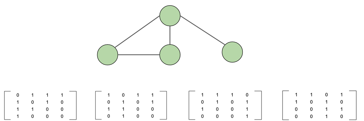
Graph representation for deep learning
When training a GNN model, we are typically required to represent 3 pieces of information about the graph. The first two pieces of information are typicial of any machine learning task and these are your x and y arrays.
In this case, the x array is any additional metadata about the node or graph (if performing graph classification) being analysed. For example, in a the karate club node classification task mentioned above, you might encode each persons years of experience, or belt grade in the x array to provide additional information to the model.
Similar to any classification or regression task, the y array will simply be the actual labels for the task being performed. In the case of our karate example this will just be which instructor each node is loyal to, and in the case of protein classification at a graph level, this will just be whether the graph represents and protein or not.
The final piece of information we are required to represent about the graph is the connectivity between each node (the edges basically). With the challenges posed by adjacency matrices above in mind, GNN's require a memory efficicent way to store information and relationships contained within a graph.
The most common way of representing these relationships in GNN's is creating an edge list. The edge list (illustrated below) is simply a list of tuples which maps the start and end point of each edge on the graph. The advantage of using an edge list over an adjacency matrix is that it does not store information about relationships that don't exist. For example if there is no edge between two nodes, this will still be stored as an entry in an adjacency matrix, which is memory inefficent.
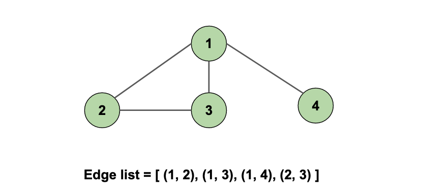
Once we have created the x, y, and edge list arrays, the training process is simply a case of wrapping these 3 arrays up as a "graph" object and passing them through the modelling architecture.
How do the models work?
In the same way that we have multiple types of deep learning architecures (DNN, RNN, Autencoder, etc.), we also have a variety of GNN architectures which we can use to solve our problems. Some examples include recurrent graph neural networks, graph autoencoders, spatial-temporal graph neural networks, and graph convolutional networks (GCNs).
For the purposes of this tutorial we are going to focus on the GCN architecture as it is the most widely used GNN architecture at the moment. However, if you wish to learn more about the other types of GNN architecures mentioned above, I would recomment the "Taxonomy of Graph Neural Networks" section of A Comprehensive Survey on Graph Neural Networks by Zonghan Wu, Shirui Pan, Fengwen Chen, Guodong Long, Chengqi Zhang & Philip S. Yu
Those of you familiar with image classification will be aware of convolutional neural networks (CNNs). These architectures were originally based on the mathematical idea of convolution is essentially an integral that expresses the overlap as one function passes over another. However, in the field of computer science and image processing this idea of convolution can be thought of as iteratively analysing small portions of an input space (e.g. 3x3 pixels across an input image) through what is known as a convolution window to extract local features. These local features are further contextualised within the input (an image usually) by merging adjacent feature maps in the space through a process called pooling.
This process then essentially creates a condensed representation each section of the image which can then be flatted and analysed by a traditional dense architecture. Figure 6 illustrates a simple example of convolution applied to a 9x9 input space.
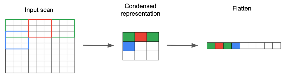
In GNN's the idea of using convolution is not too different. Rather than condensing sections of an image based on the pixels in it's locallity, GCN's iterate over each node in the graph and create a condensed representation of each node based on the features of the nodes it is conneced to.
Once we have a condensed representation of each node, we can simply pass these vectors through a dense architecture to make predictions of the properties of a given node.
The example below provides a very simple illustartion how a GCN will create a vector representation of a node (the blue one) based on the features of it's surrounding nodes.
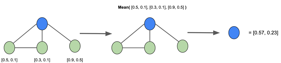
It's worth noting that the idea of a GCN in graph modelling isn't too dissimilar from a sentence transformer in natural language processing. Where a sentence transformer will convert a sentence into a vector representation which we can pass through some classification model or clustering algorithim, a GCN will convert a node on a graph to a similar vector representation which can be passed through a dense deep learning architecture to perform some classification.
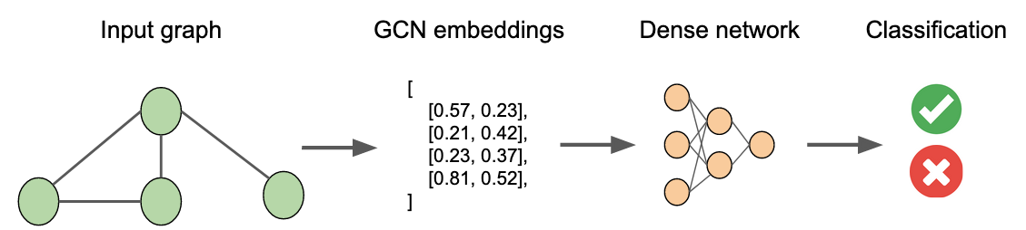
Classifying soccer player positions from passing networks
Now that we have a bit of an understanding on what GNN's are how they can be work, lets get stuck into an example.
In the example detailed below I will demonstrate how we can use GCN to classify players from the Italian mens national team positions based on their average passing position and passing network using a subset of 4 matches played at Euro 2020.
It's worth pointing out that while the below section summarises the steps and code used as part of this example, the jupyter notebooks provided in my GitHub repo provide all the code required to replicate the results, so feel free to clone that and use it as a basis for your own modelling.
The dataset
The dataset used as part of this example will be a subset of the Statsbomb open event dataset. This dataset match and detailed event (passes, shots, etc) data for over 1,000 matches from 2003 through 2021.
Getting access to the data is very straightforward, you can simply clone the StatsBomb open data repository to your local machine.
Data preparation
Transforming the source data
Before we can get into any modelling, we must first transform the Statsbomb event data into a format we can convert into a passing network. The coding required to perform all the transformations is quite long (and could even be a blog post in itself!), so in the interest of keeping this tutorial short, I have created a separate notebook inside the GitHub repo that accompanies this tutorial. The data processing steps performed in that notebook can be summarised as:
-
Import the data and extract passing events for Euro 2020
-
For each passing event store the players who passed and received the ball, their positions, and the passers location on the pitch
-
Figure out which position each player started the match in and encode it as an integer (for modelling)
-
Remove any players who had little involvement in the match (these cause noise)
-
Split into training, testing, and validation sets
| match_id | team_id | from_player_id | from_position | to_player_id | to_position | from_position_x | from_position_y | from_position_encoded |
|---|---|---|---|---|---|---|---|---|
| 3795506 | 914 | 7788 | Forward | 3166 | Midfield | 60.0 | 40.0 | 1 |
| 3795506 | 914 | 3166 | Midfield | 11514 | Defender | 48.0 | 35.7 | 3 |
| 3795506 | 914 | 11514 | Defender | 7173 | Defender | 39.2 | 68.4 | 0 |
| 3795506 | 914 | 7173 | Defender | 6954 | Defender | 25.3 | 46.4 | 0 |
| 3795506 | 914 | 6954 | Defender | 7173 | Defender | 23.9 | 18.6 | 0 |
| 3795506 | 914 | 7173 | Defender | 7036 | Goalkeeper | 16.2 | 44.3 | 0 |
| 3795506 | 914 | 7788 | Forward | 7024 | Midfield | 60.0 | 40.0 | 1 |
Once the steps above are completed we will have 4 CSV files which contain the training, testing, and modelling data. Each file follows a the same format to what is detailed in the example table above and correspond to the following Euro 2020 matches:
-
Training: Italy v England & Italy v Spain
-
Validation: Italy v Belguim
-
Testing: Italy v Austria
Converting to graph for modelling
Once we have the datasets imported (via pandas), the next step required is to convert these dataframes into the model format discussed in section 1. To do this (see code snippet below) we will define a function called create_graph_from_dataframe which will take a pandas DataFrame as input and:
-
Use the networkx library to convert this DataFrame to a networkx graph object
-
Use PyTorch Geometric's
from_networkxfunction to extract the edge list from this graph. -
From here, we create the graphs
xfeatures (average player passing position). To do this we simply iterate through each node (i.e. player) in the graph and calculate their averagefrom_position_xandfrom_position_yusing pandas. -
Similar to step 3, we will add the
ylabels to the PyTorch Geometric graph by iterating across each node and pulling the encoded players position from the source data -
Finally we just handle some type conversions and add the
player_idas a separate feature on the graph which helps with plotting later.
Once we have that function created, we can very easily pass our 4 training/testing/validation files through this function to create the input data for our model.
def create_graph_from_dataframe(dataframe: pd.DataFrame):
  # first create a network x representation of the graph from the pandas dataframe
  match_network_x_graph = nx.from_pandas_edgelist(
      dataframe, source="from_player_id", target="to_player_id"
  )

  # then convert that to a pytorch geometric graph
  graph_for_modelling = from_networkx(match_network_x_graph)


  # create our x features (player mean passing positions)
  graph_for_modelling.x = torch.tensor(
    list(
      {
          n:list(dataframe.loc[
              dataframe["from_player_id"]==n,
              ["from_position_x", "from_position_y"]
          ].mean()) for n in match_network_x_graph.nodes()
      }.values()),
      dtype=torch.float
  )/100

  # create our y (target) features
  graph_for_modelling.y = torch.tensor([
      dataframe.loc[
        dataframe["from_player_id"]==n, "from_position_encoded"
    ].iloc[0] for n in match_network_x_graph.nodes()
  ], dtype=torch.long)

  # ensure the edge index/list is of the correct datatype
  graph_for_modelling.edge_index = graph_for_modelling.edge_index.type(
      torch.LongTensor
  )

  # add the player id as a feature to help us when plotting later
  graph_for_modelling.player_id = [n  for n in match_network_x_graph.nodes()]

  return graph_for_modelling

modelling_train = [create_graph_from_dataframe(match) for match in [training_match_1, training_match_2]]
modelling_val = create_graph_from_dataframe(vaidation_match)
modelling_test = create_graph_from_dataframe(testing_match)
Modelling
The modelling architecture
Now that we have the input data ready to go, we can get started on our modelling by first creating our modelling architecture.
The model architecture used for this tutorial will rely on the SageConv GCN architecture proposed by Hamilton, Ying & Leskovec in their 2017 paper. This GCN architecture is a more robust form of GCN which is capable of handling graphs with a varying number of nodes, which is ideal for our use case (e.g. some matches might have 11 players play a role whereas others may have 15 when you include subs). Thankfully fot us, Pytoch Geometric provides support for this model out of the box so we can easily include it in our classification architecture.
To create the model we will first define some model parameters such as the number of units in our hidden layers and the number of positions we want to be able to classify.
From here, we will defin a GCN class which will include an __init__ that defines the types of layers our architecture will include before defining a forward function which is essentially our model. Those of you who have used PyTorch or Keras before will recognise that how we create GNN's here is basically exactly the same as how you would define a standard deep learning model using those frameworks.
In our architecture we start off with the SageConv GCN architecture, before passing the output of SageConv through two standard dense layers which in turn proceeds to the classification layer with the final classification being based on the softmax output of this layer (see my blogpost on activation functions if you are unfamiliar with the softmax function).
To avoid any overfitting on the training set, we also include a couple of dropout layers. This step is particuarly important when dealing with such a small dataset.
from torch.nn import Linear
import torch.nn.functional as F
from torch_geometric.nn import SAGEConv

NUM_FEATURES = modelling_train[0].x.shape[1]
NUM_CLASSES = len(training_match_1["from_position_encoded"].drop_duplicates())
HIDDEN_LAYER_SIZE = 256

class GCN(torch.nn.Module):
    def __init__(self):
        super().__init__()
        # Model layers
        self.conv1 = SAGEConv(NUM_FEATURES, HIDDEN_LAYER_SIZE)
        self.lin_1 = Linear(HIDDEN_LAYER_SIZE, NUM_CLASSES*4)
        self.lin_2 = Linear(NUM_CLASSES*4, NUM_CLASSES)


    def forward(self, data):
        # separate data from the input
        x, edge_index, batch = data.x, data.edge_index, data.batch

        # The architecture itself
        x = self.conv1(x, edge_index)
        x = F.relu(x)
        x = F.dropout(x, p=0.5, training=self.training)

        x = self.lin_1(x)
        x = F.relu(x)
        x = F.dropout(x, p=0.5, training=self.training)

        x = self.lin_2(x)

        return F.log_softmax(x, dim=1)
Training
Once we have the the model architecture set up, we can start training our model. To do this we first load the model architecture defined by our GCN class above before defining the optimizer (Adam) and loss function (categorical cross entropy) for our model.
From here we define two functions (see below) train_model and evaluate_model. The train_model function will simply iterate through the graphs in our training dataset (2 matches) and update the weights in the model (the same way we would train any other model). The evaluate_model will simply take in some test/validation data and make a prediction for it using the model, the function will then calculate the accuracy and loss for the model on the given dataset.
model = GCN().to(device)
optimizer = torch.optim.Adam(model.parameters(), lr=0.001)
criterion = torch.nn.CrossEntropyLoss()

def train_model(train_data):
    model.train()
    for data in train_data:
      out = model(data) # Perform a single forward pass.
      loss = criterion(out, data.y)  # Compute the loss.
      loss.backward()  # Derive gradients.
      optimizer.step()  # Update parameters based on gradients.
      optimizer.zero_grad()  # Clear gradients.

    return model

def evaluate_model(test_data):
    model.eval()
    correct = 0
    total_samples = 0

    model_outputs = []
    targets = []
    for data in test_data:
      model_output = model(data)
      predicted_class = model_output.argmax(dim=1)

      correct += int((predicted_class == data.y).sum())
      total_samples += len(data.y)

      # store these to get the loss
      model_outputs.extend(model_output.tolist())
      targets.extend(data.y.tolist())

    accuracy = correct/total_samples
    loss = criterion(torch.tensor(model_outputs), torch.tensor(targets))

    return accuracy, loss
With these functions defined we can train the model by passing in our training and validation datasets as demonstarted below. In my example I trained over 3,000 epochs, however if you had more matches in your training set, this number could be reduced significantly I would imagine.
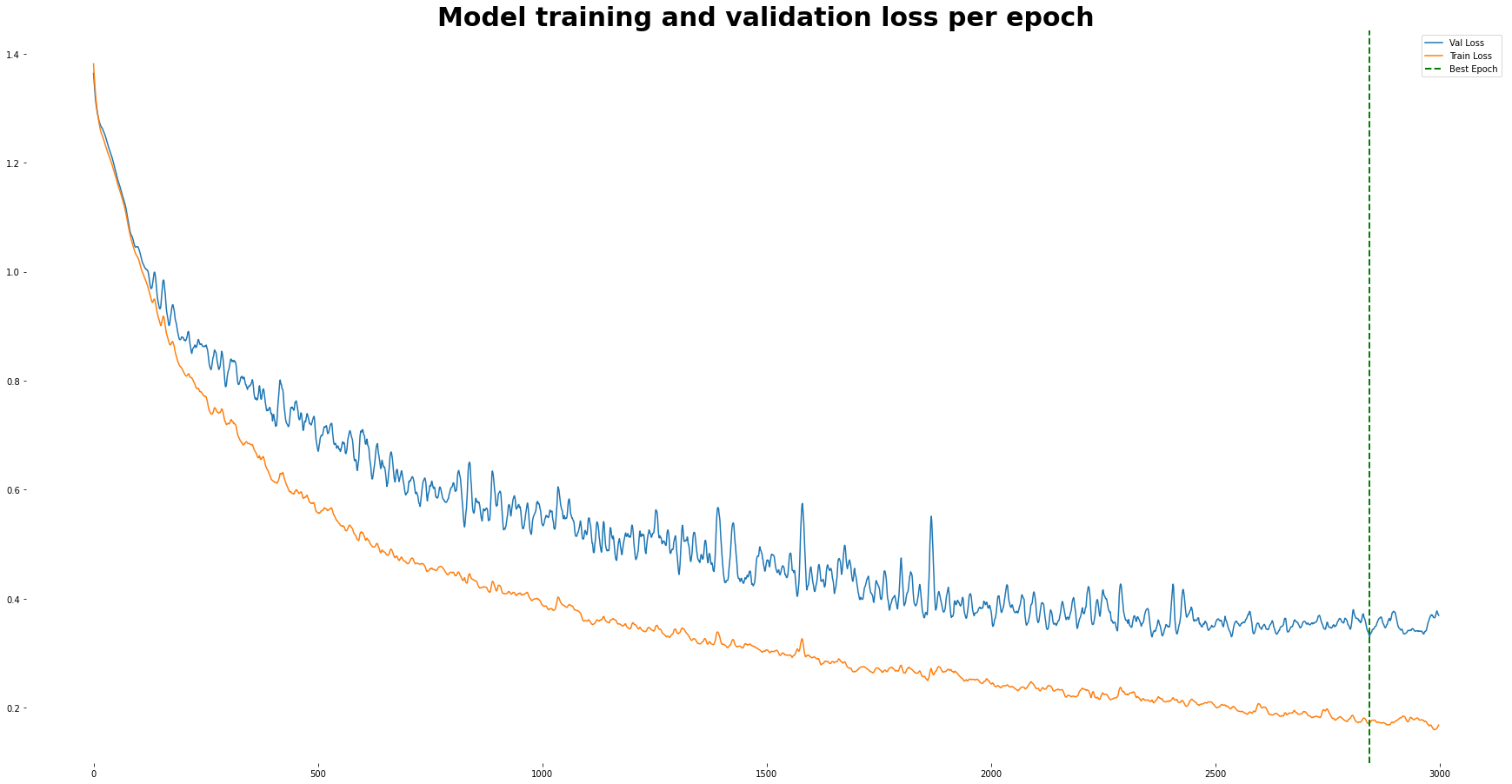
At each epoch we save the training and validation loss, and to prevent overfitting on the training set compare the validation loss to all orevious validation losses and if the current loss is the lowest we've seen, we will save the model locally. This means that once we have completed the training process we will be left with the model which performed best on the unseen validation dataset.
train_accuracies = []
validation_accuracies = []
validation_losses = []
train_losses = []
for epoch in range(1, 3000):
    train_accuracies = []
    model = train_model(modelling_train)

    train_acc, train_loss = evaluate_model(modelling_train)
    train_losses.append(train_loss)
    val_acc, val_loss = evaluate_model([modelling_val])
    validation_losses.append(val_loss)


    train_accuracies.append(train_acc)
    validation_accuracies.append(val_acc)

    # save the model if it is the better than any previous ones
    if val_loss.item() <= min(validation_losses).item():
      torch.save(model, "best_model.pkl")
    if epoch % 50 == 0:
      print(f'Epoch: {epoch}, Train Acc: {train_acc:.4f}, Train Loss: {train_acc:.4f}, Val Acc: {val_acc:.4f}, Val Loss: {val_loss:.4f}')

best_validation_loss = min(validation_losses)
best_epoch = validation_losses.index(best_validation_loss)
accuracy_at_best_epoch = validation_accuracies[best_epoch]
print(f"The best result was achieved after {best_epoch} epochs with a validation accuracy of {accuracy_at_best_epoch} and a loss of {best_validation_loss}")
The graph below illustrates the training and validation loss throughout the training process. As you can see, the model reached it's optimum validation loss after roughly 2,800 epochs and this corresponded to an validation accuracy of ~90%.
Evaluation
Now that we have a GCN model trained, we can go ahead and make some predictions based on our unseen data from the Italy v Austria round of 16 matchup.
To make these predictions we simply load the best model we had saved fromfrom the training process before simply passing the test data through this model (as demonstrated below). This will return the a probability for each node and class in the testing data and will just use the argmax function to get the class with the highest probabilty before computing the accuracy based on the number of correctly predicted classes.
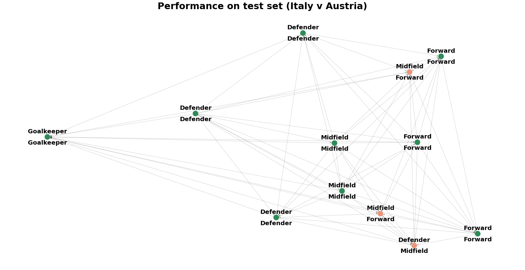
In this case our model achieved a accuracy score of 75% based on the 12 players who performed a meaningful number of passes in the match.
# load the model
best_model = torch.load("best_model.pkl")

# predict the output
model_output = model(modelling_test)
predicted_class = model_output.argmax(dim=1)

# calculate the accuracy
int((predicted_class == modelling_test.y).sum())/len(modelling_test.y)
Taking a closer look at where the model went wrong in the visual below (code for creating this can be found in the supporting notebook) which illustrates each players actual position (above) and predicted position (below), we can see that the model (perhaps unsurprisingly) did a great job at detecting defenders and forwards for the most part, but struggled with classifying advanced midfielders and wing backs. This is probably no surprise as I too would struggle to correctly classify some of those nodes correctly if the below graph was given to me with no labels. However, we could try improve this going forward by adding more matches to our training set.
Conclusion
Closing thoughts
In this blogpost, I summarised the area of graph neural networks before going through through how we can create create a simple player position prediction using a graph convolutional network within the pytorch framework on the Statsbomb open event dataset.
This model achieved 90% accuracy on the validation data but only a modest 75% accuracy on the unseen testing data. However given the lack of training data (only two matches) this performance is somewhat understandbale.
I hope that the code and summaries provided in this tutorial as well as in the accompanying GitHub repositiory will provide you with a starting point for training your own GNNs on similar data in the future. Feel free to also use some of the ideas I mention below in the future directions section as exercises to get some hands on experience with the ideas discussed above.
If you would like to learn more about graph neural networks, I would strongly recommend DAIR.ai's GitHub repo which provides and abundance of useful resources on this topic.
Future directions
While creating the material for this blogpost I had a few ideas on things I would like to try to improve the model. I have listed these below in case anyone reading this wants to take any of the material further:
-
Pick a different team (or teams) and try train the same model to see how different the results are. I would expect that the model would perform better for less fluid teams. I have included a dataset (
data/full_pass_network_data.csv) in the Git repo that includes the passing events off all teams from Euro 2020, you can filter this down to a particular team and go from there. -
Rather than focusing on one team in particular, see can you use the full dataset I provide to build a generalised position predictior for all teams at the euros, you could even include a team identifier in the graphs
xfeatures to improve this model. -
While this tutorial was meant to show how we can use GNN's to build a model, I suspect that we could have got similar, if not better accuracy with a simpler model. See if you can train a simple SVM based only on the players avaerage passing positions and compare that to the accuracy of the model from this tutorial.